Mathematical_Numerical_Methods_MOC
Mathematical and Numerical Methods for Astrophysics - Map of Content
A.Y. 2025/2026, Prof. Michela Mapelli, University of Padova. Master’s-level first-semester course in the Astrophysics and Cosmology programme. Exam scheduled 24 June 2026 (written, four exercises in Python on a fixed time slot, scripts and plots uploaded).
This is the toolbox course. it does not teach me astrophysics. It teaches me how to do astrophysics on a computer. every time I will integrate an N-body system, fit a CMB peak, draw mock binaries from a population, deconvolve a spectrum, or solve a Friedmann equation numerically, this is the course that taught me how. it underwrites the python in [[Observational_Cosmology_MOC]], the simulations in [[Lab_High-Energy_MOC]], and the equation-solving I do throughout [[General_Relativity_MOC]] and [[Fundamentals_Astrophysics_Cosmology_MOC]].
the course has two faces, married together by the title. the mathematical face teaches the linear algebra (eigenvalues, QR decomposition, Gram-Schmidt) and the analysis (Fourier series, finite differences, error propagation) that justify the algorithms. the numerical face is the algorithms themselves: Gauss elimination, Newton-Raphson, Runge-Kutta, leapfrog, Monte Carlo, FFT. for every block below I keep both faces in view: what is the math? and what is the algorithm?
the question this course is trying to answer
how do I solve, on a computer, a problem that has no closed-form solution?
every analytical problem I have ever met in physics had a clean answer: harmonic oscillator, Kepler orbit, hydrogen atom. real research never works that way. the three-body problem has no closed form. Friedmann with $\Omega_m, \Omega_\Lambda, \Omega_r$ all non-zero has no closed form. fitting Planck data to $\Lambda$CDM has no closed form. an N-body simulation of a globular cluster has no closed form. the universe is a numerical problem.
this course is the answer to given a problem with no analytical solution, what tool do I reach for, and how do I trust its output? every algorithm I learn comes packaged with two questions: how accurate is it, and how fast is it. the tradeoff between accuracy and speed is the recurring theme.
the chain of objects, what we will build
Mapelli’s notes follow a deliberate ladder. we start with the simplest possible problem (a linear equation) and climb to the most complex (a partial differential equation), and at each rung we meet a new class of algorithm:
\[\text{linear system} \to \text{nonlinear root} \to \text{derivative} \to \text{integral} \to \text{ODE} \to \text{N-body} \to \text{PDE} \to \text{fit and transform}\]every later problem reduces, at the algorithm level, to a sequence of earlier ones. an ODE solver calls a derivative. an N-body integrator calls an ODE solver in a loop. a PDE solver calls finite differences and a linear solver. a fit calls a linear solver. an FFT calls integration. so the order is not arbitrary. it is the dependency graph of the toolbox.
reference texts
- Mapelli, Numerical Methods for Astrophysics - the official course notes (
numerical_methods_mapelli.pdf). the spine I follow lecture by lecture - Newman, Computational Physics - the textbook Mapelli’s notes are inspired by, deeper treatments of every algorithm
- Kiusalaas, Numerical Methods in Engineering with Python - the second textbook the course leans on, more code-forward
- Press, Teukolsky, Vetterling, Flannery, Numerical Recipes (3rd ed., C++ but algorithms are universal) - the encyclopedic reference, reach for it when an algorithm has a subtle case
- Strang, Linear Algebra and Its Applications - when I need linear algebra intuition, not algorithms
- Axler, Linear Algebra Done Right (in source folder) - proofs-first linear algebra companion
how to use this map
every blue link below drops into a single concept zettel. the structure I recommend to the future me reading this two weeks before the exam:
- read this MOC top to bottom to recover the dependency graph
- for each block, read the linked zettels in order, since they build on each other
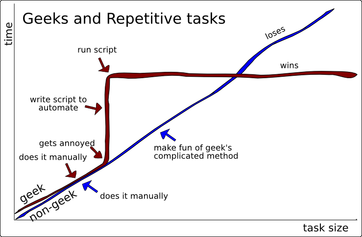
- for each block, write one toy script that implements the central algorithm from scratch - this is the only way the algorithm sticks
- practise on the past exam papers in
05_Projects/Exam/First Year/Math Numerical Methods Exam 2026/, since the exam is the practice
every zettel follows the same pattern: motivation, math, algorithm in pseudocode, accuracy and stability remarks, when to use it, common bugs.
block 0 - course frame
before any algorithm, just what is this course, what is the exam, and how do I think about a numerical problem.
- [[Math Numerical Methods course intro]] - what the course is, who teaches it, how it connects to the other MOCs
- [[Math Numerical Methods exam rules]] - four-exercise written exam, Python scripts uploaded, time pressure, rubric
- [[Math Numerical Methods equation sheet]] - every formula I might want, organized for fast lookup
- [[Numerical problem solving workflow]] - the meta-skill: define the math, pick the algorithm, validate with a known case, profile, productionize
block 1 - computing setup, the python toolbox
before any algorithm, the infrastructure. this is the unglamorous but critical part: a numerical method is only as useful as my ability to run it, debug it, and produce a publication-quality plot at the end. astrophysicists live in a python ecosystem (numpy + scipy + matplotlib + astropy + pandas), and Mapelli’s notes spend the first three chapters teaching me to be fluent in it.
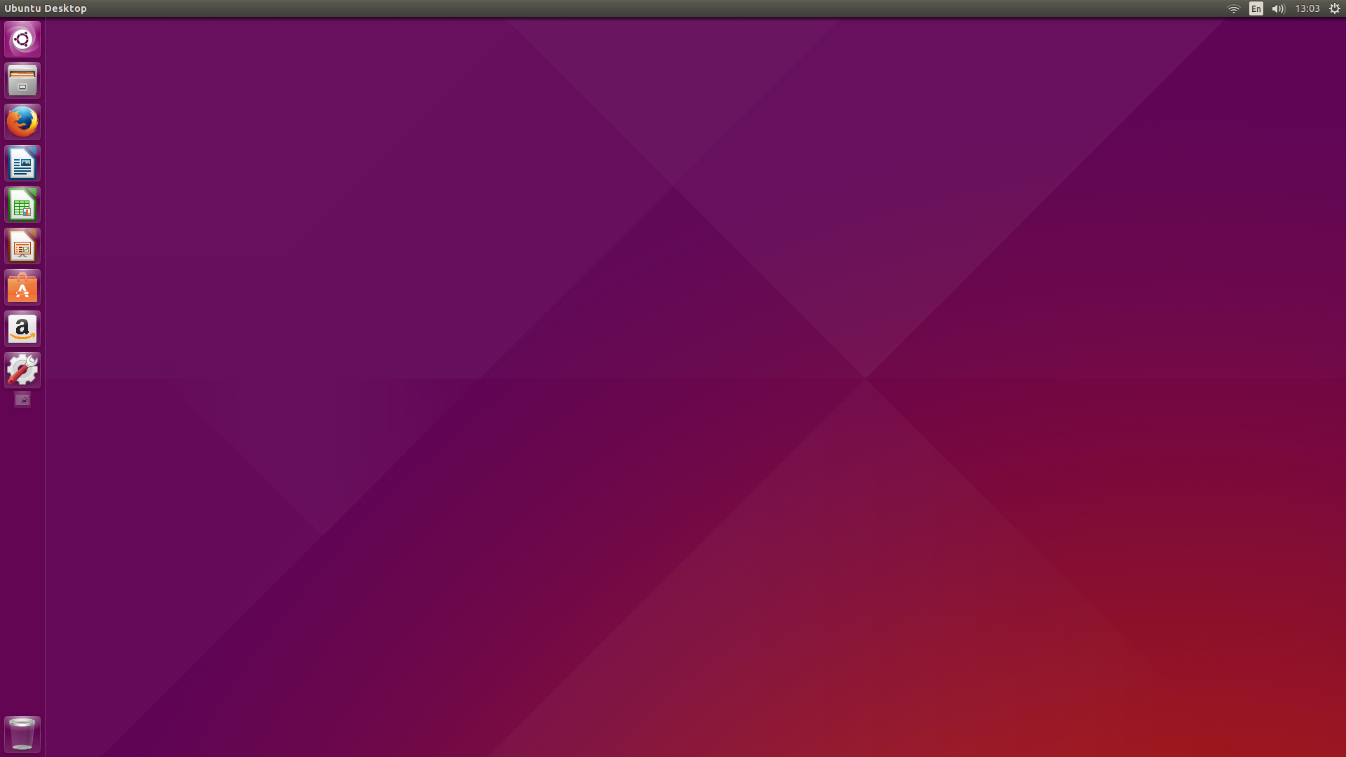
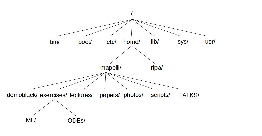
- [[Linux for the astrophysicist]] - bash, file system, pipes, redirection,
grep,find,ssh, the few commands I actually need - [[Python language essentials]] - variables, types, lists vs tuples vs dicts, control flow, functions, file I/O - the fast-path version of chapter 2
- [[Numpy arrays vs Python lists]] - the single most important python performance lesson: vectorize. the difference between
for i in range(N): a[i] = ...anda = np.where(...)can be 100× - [[Matplotlib plotting essentials]] - scatter, line, log axes, histogram, 2D histogram, subplots, what makes a figure good
- [[Scipy and astropy quick reference]] -
scipy.optimize,scipy.integrate,scipy.interpolate,scipy.fft,astropy.units,astropy.io.fits - [[Pandas for tabular astrophysics data]] - DataFrames, reading CSV/FITS, groupby, the catalog workflow
- [[The conda environment]] - environments, package isolation, why I keep one per project
block 2 - accuracy and speed, the recurring tradeoff
every algorithm in this course has two numbers attached: how accurate is it (error scaling with step size $h$), and how fast is it (operation count scaling with problem size $N$). these are not independent, usually I trade one for the other. this block teaches me to read the tradeoff.
- [[Floating point representation and rounding errors]] - IEEE 754, machine epsilon $\epsilon \sim 2.2\times 10^{-16}$, why $0.1 + 0.2 \neq 0.3$, accumulated rounding $\sim \sqrt{N}\,\epsilon$
- [[Truncation error and order of accuracy]] - Taylor series, $O(h^p)$ scaling, why central differences are second-order while forward are first-order
- [[Roundoff vs truncation balance]] - the U-shaped error curve, optimal step size $h_{\rm opt} \sim \sqrt{\epsilon}$ for first-derivative finite differences
- [[Computational complexity and speed]] - Big-O notation, $O(N^3)$ for Gauss elimination, $O(N^2)$ for matrix-vector, $O(N\log N)$ for FFT, $O(N\log N)$ for sorting
- [[Vectorization and python speed]] - why python loops are slow, what numpy does under the hood, when to call out to scipy or compiled code
block 3 - linear systems, $A\mathbf{x} = \mathbf{b}$
the problem. given a square matrix $A$ and a known vector $\mathbf{b}$, find the unknown vector $\mathbf{x}$. this is the workhorse of numerical physics: it appears in fitting (least squares is a linear system), in PDE discretization (finite differences become a sparse linear system), in eigenvalue problems (a step in the QR algorithm), and in countless one-off problems.
physical question this block answers: how do I invert a matrix and solve a linear system without inverting the matrix?
- [[Gauss elimination]] - the classical algorithm, $O(N^3)$, the row-reduction-then-back-substitution pattern
- [[Partial pivoting]] - when the algorithm fails (zero or tiny pivots) and how to fix it by row-swapping
- [[LU decomposition]] - $A = LU$, factor once and reuse for many right-hand sides, the forward-then-backward substitution
- [[Gauss-Seidel iteration]] - iterative method, $O(N^2)$ per step, when it converges (diagonally dominant matrices), when it beats direct methods (sparse $A$)
- [[Pros and cons of linear solvers]] - the decision tree: dense vs sparse, one RHS vs many, well-conditioned vs ill-conditioned, big vs huge
- [[Matrix inverse via linear systems]] - never invert a matrix directly: solve $AX = I$ column by column instead
block 4 - eigenvalues and matrix factorization
a special class of problem: find $\lambda, \mathbf{v}$ such that $A\mathbf{v} = \lambda\mathbf{v}$. eigenvalues encode physics (normal modes, principal components, stationary states) and they encode algorithm convergence (a fixed-point iteration converges iff the iteration matrix has spectral radius $< 1$). this block is the mathematical core of the course: it goes deepest into linear algebra theory.
physical question this block answers: how do I find the natural axes of a linear transformation, in a way that is numerically stable?
- [[Gram-Schmidt orthogonalization]] - turn a basis into an orthonormal basis by projection-and-subtract, with the modified version that preserves stability
- [[QR decomposition]] - every matrix factors as $A = QR$ with $Q$ orthogonal and $R$ upper triangular, Gram-Schmidt gives one explicit construction
- [[QR algorithm for eigenvalues]] - iterate $A_{k+1} = R_k Q_k$ where $A_k = Q_k R_k$, converges to a diagonal matrix with eigenvalues on the diagonal
- [[Power iteration]] - the simplest eigenvalue method, finds the dominant eigenvalue/vector by repeated matrix-vector products
- [[Matrix diagonalization $A = VDV^T$]] - for symmetric $A$, the eigenvector matrix is orthogonal and $V^TAV = D$, the geometric meaning of “principal axes”
block 5 - solution of non-linear equations, root finding
next rung up: I want $f(x) = 0$ for a function $f$ I cannot solve analytically. equilibria of dynamical systems are roots, intersections are roots, optimization first-order conditions are roots. four classical algorithms with very different tradeoffs.
physical question this block answers: given a function $f$ that I can evaluate but not invert, how do I find $x$ such that $f(x) = 0$?
- [[Relaxation method]] - rewrite $f(x) = 0$ as $x = g(x)$ and iterate $x_{n+1} = g(x_n)$, converges if $\lvert g’(x^*)\rvert < 1$
- [[Overrelaxation]] - accelerate relaxation by overshooting: $x_{n+1} = x_n + \omega(g(x_n) - x_n)$ with $\omega > 1$
- [[Bisection method]] - bracket a root and halve the interval, bulletproof but slow ($O(\log_2(1/\epsilon))$ iterations to error $\epsilon$)
- [[Newton-Raphson method]] - local linearization, $x_{n+1} = x_n - f(x_n)/f’(x_n)$, quadratic convergence when it works, divergence when it doesn’t
- [[Newton-Raphson for systems of equations]] - multivariate generalization with the Jacobian, $\mathbf{x}_{n+1} = \mathbf{x}_n - J^{-1}(\mathbf{x}_n)\mathbf{f}(\mathbf{x}_n)$
- [[Choosing a root finder]] - bracket-then-Newton hybrid, when bisection wins, when Newton fails (multiple roots, flat derivative)
block 6 - numerical derivatives
derivatives are easy in calculus and surprisingly subtle on a computer. the natural definition $f’(x) \approx [f(x+h) - f(x)]/h$ has two sources of error: truncation (finite $h$) and roundoff (cancellation in the numerator). they fight each other, and the resolution is the U-shaped error curve.
physical question this block answers: given a function $f$ that I can evaluate at points, how do I estimate $f’(x)$, and how small should $h$ be?
- [[Forward backward and central differences]] - the three first-derivative formulas, errors $O(h)$, $O(h)$, $O(h^2)$ from Taylor
- [[Second derivatives]] - $f’‘(x) \approx [f(x+h) - 2f(x) + f(x-h)]/h^2$, $O(h^2)$ accuracy
- [[Partial numerical derivatives]] - finite differences in each direction, building the Jacobian column by column
- [[Derivatives of noisy data]] - when $f$ has measurement noise, finite differences amplify the noise, the fix is smoothing or fitting first, differentiating second
- [[Optimal step size for derivatives]] - $h_{\rm opt} \sim \sqrt{\epsilon}$ for forward differences, $h_{\rm opt} \sim \epsilon^{1/3}$ for central, where $\epsilon$ is the relative error in $f$
block 7 - integration of functions
the inverse direction: given $f$, I want $\int_a^b f(x)\,dx$. integration is much more numerically stable than differentiation (it averages noise instead of amplifying it), and admits a richer family of algorithms.
physical question this block answers: given a function $f$, how do I compute its integral over a finite range, and how do I do this in many dimensions?
- [[Trapezoidal rule]] - straight lines between samples, $O(h^2)$ error, the simplest non-trivial quadrature
- [[Simpson’s rule]] - parabolas between triplets of samples, $O(h^4)$ error, the workhorse for smooth integrands
- [[Trapezoidal rule error estimate]] - error is bounded by the second derivative, how to know how many points I need
- [[Monte Carlo integration mean value method]] - integral as expectation, $\int f \approx (b-a)\langle f \rangle$, error $\sim 1/\sqrt{N}$ regardless of dimension
- [[Multidimensional Monte Carlo integration]] - the dimension-curse breaker: in $d \geq 4$, MC beats grid quadrature
- [[Importance sampling]] - sample from $g(x)$ instead of uniform, weight by $f/g$, reduces variance dramatically when $g \approx f/\lVert f\rVert$
- [[Built-in scipy integrators]] -
scipy.integrate.quad,scipy.integrate.simps, when to trust them
block 8 - random numbers and Monte Carlo
every Monte Carlo method is built on a stream of pseudo-random numbers. this block teaches me how that stream is made, why it is pseudo, how to draw from arbitrary distributions, and how to verify my draws.
physical question this block answers: given a uniform pseudo-random stream, how do I draw $N$ samples from an arbitrary distribution $P(x)$?
- [[Pseudo-random number generators]] - linear congruential, Mersenne Twister, why “random” is deterministic, periodicity
- [[Random number seeds]] - reproducibility for science,
np.random.seed, the conventions in publishable code - [[Inverse transform sampling]] - invert the CDF: if $u \sim U(0,1)$ then $F^{-1}(u) \sim P$, the textbook method, requires invertible CDF
- [[Box-Muller transform for Gaussian random numbers]] - sample two uniforms, return two normals, the polar-coordinate trick
- [[Rejection sampling]] - bounding-box method, accept if uniform $y < P(x)$, works for any pdf, efficiency = ratio of areas
- [[Verifying random samples]] - histogram against expected pdf, Kolmogorov-Smirnov test, mean and variance checks
block 9 - ordinary differential equations
now we get to the heart of numerical astrophysics. an ODE is $\dot{\mathbf{y}} = \mathbf{f}(\mathbf{y}, t)$ with initial condition $\mathbf{y}(t_0) = \mathbf{y}_0$. this is every dynamical problem: orbits, stellar structure, accretion disk evolution, expansion of the universe. the algorithms differ in accuracy, speed, and what they conserve.
physical question this block answers: given a system $\dot{\mathbf{y}} = \mathbf{f}(\mathbf{y}, t)$, how do I evolve it from $t_0$ to $t_f$ accurately enough to trust the result?
- [[Euler method]] - $\mathbf{y}_{n+1} = \mathbf{y}_n + h\mathbf{f}(\mathbf{y}_n, t_n)$, $O(h)$, the forward-Euler scheme - the simplest possible integrator and a teaching tool more than a production one
- [[Runge-Kutta 2 midpoint method]] - half-step prediction then full-step correction, $O(h^2)$
- [[Runge-Kutta 4 method]] - four-stage scheme, $O(h^4)$, the workhorse general-purpose integrator
- [[Systems of ODEs and higher-order ODEs]] - turn $y’’ = f(y, y’, t)$ into a 2D system $(y, v)$ with $v = y’$
- [[Leapfrog integrator]] - symplectic, drift-kick-drift, conserves energy on average for Hamiltonian systems, the integrator of choice for orbital and N-body problems
- [[Fourth-order Hermite predictor-corrector]] - uses both $\mathbf{f}$ and $\dot{\mathbf{f}}$, $O(h^4)$ with two function evaluations, the standard for collisional N-body
- [[Adaptive step size control]] - error estimate from comparing two methods, adjust $h$ to keep error tolerable, why fixed-step integrators fail near close encounters
- [[Modified midpoint method]] - Gragg’s method, the building block of Bulirsch-Stoer
- [[Bulirsch-Stoer extrapolation]] - Richardson extrapolation in step size, accuracy that grows with iteration, expensive but lethal for smooth problems
- [[Initial value vs boundary value problems]] - IVPs evolve forward, BVPs constrain at both ends, completely different algorithm families
- [[Shooting method]] - turn a BVP into a root-finding-plus-IVP problem: shoot, miss, adjust the initial slope, shoot again
block 10 - the astrophysical N-body problem
an N-body problem is just a special ODE: $\ddot{\mathbf{r}}i = -G\sum{j\neq i} m_j (\mathbf{r}_i - \mathbf{r}_j)/\lvert\mathbf{r}_i - \mathbf{r}_j\rvert^3$. but it is the astrophysical ODE, every gravitational simulation, from the solar system to a galaxy cluster, is one. and it has special structure (Hamiltonian, energy-conserving, scale-free) that the integrator should respect.
physical question this block answers: given $N$ massive particles interacting gravitationally, how do I evolve them for a long time without the energy drifting?
- [[Astrophysical N-body problem formulation]] - equations of motion, units (often $G = 1$), softening for close encounters
- [[N-body with Euler vs midpoint vs leapfrog]] - energy conservation comparison: Euler drifts secularly, midpoint drifts slower, leapfrog oscillates around the true energy without a drift - the symplectic-integrator demonstration
- [[Energy conservation as a diagnostic]] - track $\Delta E/E$ vs time, for a Hamiltonian system, the integrator’s quality is read directly off this number
- [[Collisional vs collisionless N-body]] - collisional (globular clusters, $N \lesssim 10^6$, every pair matters, Hermite), collisionless (galaxies, $N \gtrsim 10^9$, tree codes, particle-mesh)
- [[Adaptive timesteps near close encounters]] - why a binary needs a smaller step than the rest of the cluster, individual timesteps and block-step schemes
- [[The Pythagorean three-body problem]] - three masses $3, 4, 5$ at the apexes of a 3-4-5 triangle, classic test of N-body integrators, behaves chaotically with a final escape
block 11 - partial differential equations
the next rung up from ODEs: now the unknown is a function of several variables, $u(x, t)$ or $u(x, y, z, t)$. PDE algorithms split by the type of equation (elliptic, parabolic, hyperbolic) and by the boundary conditions (Dirichlet, Neumann, periodic). Mapelli’s chapter is short and focused: finite-difference discretization on a grid.
physical question this block answers: how do I discretize a PDE on a grid, and how do I keep the discrete solution stable?
- [[Finite difference discretization]] - replace partial derivatives by finite differences, turn the PDE into a system of algebraic equations on grid points
- [[Boundary value PDEs and iteration]] - Laplace, Poisson, relax the grid until the residual is small (Gauss-Seidel on the grid)
- [[Initial value PDEs and FTCS]] - diffusion, advection, forward-time, centered-space, explicit, simple, sometimes unstable
- [[Stability and the Courant condition]] - explicit schemes have a CFL constraint $c\Delta t/\Delta x \leq 1$ (hyperbolic) or $D\Delta t/\Delta x^2 \leq 1/2$ (parabolic), violating it makes the simulation blow up
- [[When to use implicit schemes]] - when the explicit time step is intolerably small, pay $O(N)$ per step (linear solver) instead of $O(1)$, but step further
block 12 - interpolation and extrapolation
between two known points, what is the function value? this is the everyday problem of working with tabulated data, opacity tables, stellar evolution tracks, observed spectra. the answer depends on how smooth I assume the underlying function to be.
physical question this block answers: given $f$ at $N+1$ points, what is $f$ between those points, and what error am I making?
- [[Linear interpolation]] - straight line between two points, simple and robust, $O(h^2)$ error
- [[Lagrange polynomial interpolation]] - unique degree-$N$ polynomial through $N+1$ points, the analytic form, when it works (low $N$, equispaced or Chebyshev nodes)
- [[Newton divided differences]] - same polynomial, written so I can add a new point without redoing the whole calculation
- [[Runge phenomenon]] - high-degree polynomial interpolation oscillates wildly at the edges with equispaced nodes, why polynomial fitting beyond $N \sim 5$ is dangerous
- [[Cubic spline interpolation]] - piecewise cubic, $C^2$ continuous, the right answer for smooth tabulated data
- [[Two-dimensional interpolation]] - bilinear, bicubic, structured grids vs scattered data
- [[Scipy interpolation tools]] -
scipy.interpolate.interp1d,interp2d,CubicSpline, when to trust each one
block 13 - fitting procedures
the data is noisy. the model has parameters. find the parameters that best match the data. this is the central problem of observational physics.
physical question this block answers: given $N$ noisy measurements $y_i$ at known $x_i$, what model parameters $\theta$ minimize the disagreement?
- [[Linear least squares]] - fit $y = mx + b$ by minimizing $\sum (y_i - mx_i - b)^2$, closed-form solution via normal equations
- [[Weighted least squares]] - when data points have different errors $\sigma_i$, weight by $1/\sigma_i^2$, the only sane choice for heteroscedastic data
- [[General linear least squares]] - fit $y = \sum_k \theta_k\phi_k(x)$ with arbitrary basis functions $\phi_k$, reduces to a linear system
- [[Polynomial fitting]] - special case of general LSQ with $\phi_k(x) = x^k$, same Runge phenomenon caveat as interpolation
- [[Goodness of fit and chi-squared]] - $\chi^2 = \sum (y_i - f_i)^2/\sigma_i^2$, expected $\chi^2/\nu \approx 1$ for good fit and right errors, why it tests the model and the errors simultaneously
- [[Non-linear fitting with scipy]] -
scipy.optimize.least_squares,curve_fit, the Levenberg-Marquardt algorithm, when to provide a Jacobian - [[Fitting practical recipe]] - center and scale $x$ before fitting, check residuals, never extrapolate, plot the fit on top of the data
block 14 - fourier transforms
the nicest algorithm in numerical mathematics. the FFT computes a discrete Fourier transform in $O(N\log N)$ instead of the naive $O(N^2)$. it is what makes spectral analysis, signal processing, image filtering, and convolution practical. and it is the gateway to spectral PDE solvers.
physical question this block answers: given a sampled signal in time, what frequencies is it made of, and how do I compute that fast?
- [[Fourier series math summary]] - the Fourier series for periodic functions, the Fourier transform for non-periodic, Parseval’s theorem, the convolution theorem
- [[Discrete Fourier transform]] - sampled $N$-point version, $X_k = \sum_n x_n e^{-2\pi i kn/N}$, $O(N^2)$ direct, periodic boundary
- [[Fast Fourier transform algorithm]] - Cooley-Tukey divide-and-conquer, $O(N\log N)$, the algorithm that runs the world
- [[Physical interpretation of the FFT]] - frequency bins, Nyquist frequency $f_{\rm Nyq} = 1/(2\Delta t)$, aliasing, leakage, windowing
- [[Power spectrum estimation]] - squared-magnitude FFT, why one should average over many segments (Welch’s method), the relation to autocorrelation
- [[FFT in scipy and numpy]] -
numpy.fft.fft,scipy.fft, real vs complex, conventions for normalization
block 15 - sorting and discrete algorithms
a small but unavoidable block. sorting is everywhere, finding nearest neighbors, building histograms, ranking, merging catalogs. and it is the canonical example for “complexity of an algorithm.”
- [[Sorting algorithms overview]] - bubble ($O(N^2)$), selection ($O(N^2)$), quicksort ($O(N\log N)$ average), mergesort ($O(N\log N)$ guaranteed), when each one wins, why python’s
sorteduses Timsort
block 16 - notions of machine learning in astrophysics
a one-chapter sketch, not a full treatment. modern astrophysics is increasingly ML-driven (galaxy classification, transient detection, parameter inference), and Mapelli closes the course with a teaser of decision trees as the gateway algorithm.
- [[What is machine learning]] - supervised vs unsupervised, training vs test, overfitting and the bias-variance tradeoff
- [[Decision tree classifier]] - the algorithm: split features by entropy/Gini, recurse, pros (interpretable), cons (high variance)
- [[Iris dataset and the ML hello world]] - three species of flower, four features, the canonical training-classification demonstration
- [[Interpretability vs accuracy in ML]] - why decision trees are interpretable and neural nets are not, why physicists care
the problem-class taxonomy (for the exam)
every Mapelli exam question lives in one of seven boxes. recognising the box on first read is half the battle:
| problem class | give-aways in the prompt | algorithm to reach for | block |
|---|---|---|---|
| read & visualize data | “download this file”, “plot a scatter / histogram” | np.loadtxt, plt.scatter, plt.hist, plt.hist2d |
1 |
| basic statistics | “mean”, “standard deviation”, “fit a Gaussian” | np.mean, np.std, scipy.stats |
1, 13 |
| draw random numbers | “generate $N$ samples from $P(x) = \ldots$” | inverse sampling if CDF invertible, else rejection | 8 |
| compute an integral | “calculate $\int_a^b f(x)\,dx$ using N points” | trapezoid (1D smooth), MC (high-D or random integrand) | 7 |
| find a root | “solve $f(x) = 0$” | bisection if bracketed, Newton if smooth | 5 |
| integrate an ODE | “evolve a system from $t_0$ to $t_f$ with timestep $h$” | midpoint / RK4 / leapfrog depending on Hamiltonian-ness | 9, 10 |
| fit a model | “fit $y = f(x; \theta)$” | linear LSQ if linear in $\theta$, else scipy.optimize.curve_fit |
13 |
the exam template I have on file (4 exercises) hits exactly these boxes: read-and-plot, inverse sampling, MC integration, N-body midpoint integration with energy diagnostic.
Literature & Primary Sources
Canonical and modern benchmark papers underlying the numerical methods above.
- [[Marquardt_1963_Levenberg_Marquardt_Algorithm|Marquardt (1963) - Levenberg-Marquardt Nonlinear Least Squares]] - adaptive Gauss-Newton/steepest-descent damping
- [[Virtanen_2020_SciPy_Scientific_Computing|Virtanen et al. (2020) - SciPy 1.0]] - the numerical-Python foundation underlying most of this course’s tooling
related MOCs and where this work leaks into
- [[Fundamentals_Astrophysics_Cosmology_MOC]] - every cosmology calculation that actually returns a number was done with the tools in this MOC: integrating Friedmann, computing $D_L(z)$, drawing mock CMB realizations
- [[General_Relativity_MOC]] - geodesic integration, effective-potential plots, perihelion-precession ODE solves
- [[Observational_Cosmology_MOC]] - fitting Planck data, MCMC, FFT for the matter power spectrum
- [[Lab_High-Energy_MOC]] - every detector simulation, every spectrum extraction, every ML photon classifier
- Moc - the master mind-map of the whole vault
Master Figure Index (43 Total Images)
Every single homework trajectory plot, Jacobi conservation diagnostic, exam paper card, and Mapelli algorithm figure in 07_Images/Mathematical_Numerical_Methods/ is cataloged below with direct links and pedagogical context:
| Image Asset | Diagnostic Category & Algorithmic Physics | Primary Zettel Note |
|---|---|---|
 |
Prof. Michela Mapelli lecture diagram: Algorithm flow, spatial treecode, stability region, or HPC parallelization | [[Mathematical_Numerical_Methods_MOC]] |
 |
Prof. Michela Mapelli lecture diagram: Algorithm flow, spatial treecode, stability region, or HPC parallelization | [[Mathematical_Numerical_Methods_MOC]] |
 |
Prof. Michela Mapelli lecture diagram: Algorithm flow, spatial treecode, stability region, or HPC parallelization | [[Mathematical_Numerical_Methods_MOC]] |
 |
Prof. Michela Mapelli lecture diagram: Algorithm flow, spatial treecode, stability region, or HPC parallelization | [[Mathematical_Numerical_Methods_MOC]] |
 |
Prof. Michela Mapelli lecture diagram: Algorithm flow, spatial treecode, stability region, or HPC parallelization | [[Mathematical_Numerical_Methods_MOC]] |
 |
Prof. Michela Mapelli lecture diagram: Algorithm flow, spatial treecode, stability region, or HPC parallelization | [[Mathematical_Numerical_Methods_MOC]] |
 |
Prof. Michela Mapelli lecture diagram: Algorithm flow, spatial treecode, stability region, or HPC parallelization | [[Mathematical_Numerical_Methods_MOC]] |
 |
Prof. Michela Mapelli lecture diagram: Algorithm flow, spatial treecode, stability region, or HPC parallelization | [[Mathematical_Numerical_Methods_MOC]] |
 |
Prof. Michela Mapelli lecture diagram: Algorithm flow, spatial treecode, stability region, or HPC parallelization | [[Mathematical_Numerical_Methods_MOC]] |
 |
Prof. Michela Mapelli lecture diagram: Algorithm flow, spatial treecode, stability region, or HPC parallelization | [[Mathematical_Numerical_Methods_MOC]] |
 |
Prof. Michela Mapelli lecture diagram: Algorithm flow, spatial treecode, stability region, or HPC parallelization | [[Mathematical_Numerical_Methods_MOC]] |
 |
Prof. Michela Mapelli lecture diagram: Algorithm flow, spatial treecode, stability region, or HPC parallelization | [[Mathematical_Numerical_Methods_MOC]] |
 |
Prof. Michela Mapelli lecture diagram: Algorithm flow, spatial treecode, stability region, or HPC parallelization | [[Mathematical_Numerical_Methods_MOC]] |
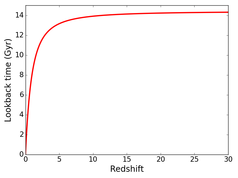 |
Prof. Michela Mapelli lecture diagram: Algorithm flow, spatial treecode, stability region, or HPC parallelization | [[Mathematical_Numerical_Methods_MOC]] |
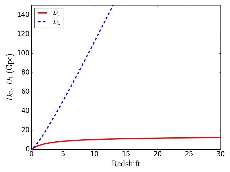 |
Prof. Michela Mapelli lecture diagram: Algorithm flow, spatial treecode, stability region, or HPC parallelization | [[Mathematical_Numerical_Methods_MOC]] |
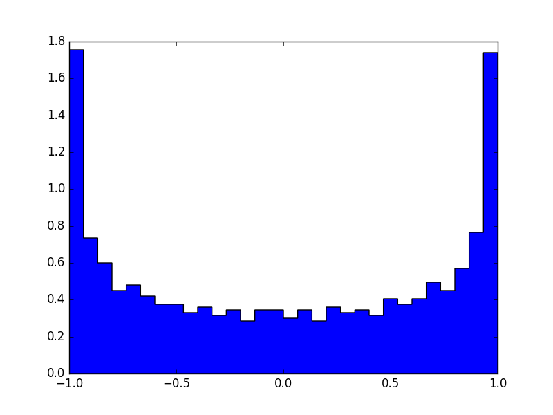 |
Prof. Michela Mapelli lecture diagram: Algorithm flow, spatial treecode, stability region, or HPC parallelization | [[Mathematical_Numerical_Methods_MOC]] |
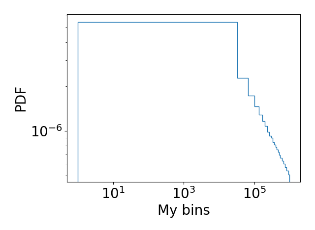 |
Prof. Michela Mapelli lecture diagram: Algorithm flow, spatial treecode, stability region, or HPC parallelization | [[Mathematical_Numerical_Methods_MOC]] |
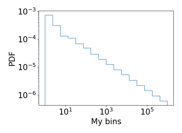 |
Prof. Michela Mapelli lecture diagram: Algorithm flow, spatial treecode, stability region, or HPC parallelization | [[Mathematical_Numerical_Methods_MOC]] |
 |
Prof. Michela Mapelli lecture diagram: Algorithm flow, spatial treecode, stability region, or HPC parallelization | [[Mathematical_Numerical_Methods_MOC]] |
 |
Prof. Michela Mapelli lecture diagram: Algorithm flow, spatial treecode, stability region, or HPC parallelization | [[Mathematical_Numerical_Methods_MOC]] |
 |
Prof. Michela Mapelli lecture diagram: Algorithm flow, spatial treecode, stability region, or HPC parallelization | [[Mathematical_Numerical_Methods_MOC]] |
 |
Prof. Michela Mapelli lecture diagram: Algorithm flow, spatial treecode, stability region, or HPC parallelization | [[Mathematical_Numerical_Methods_MOC]] |
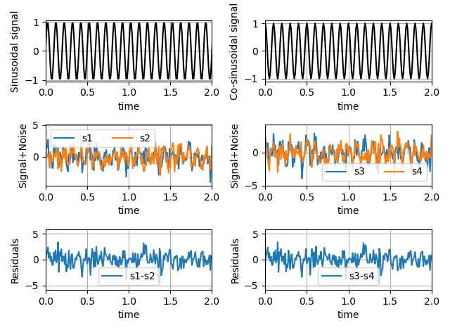 |
Prof. Michela Mapelli lecture diagram: Algorithm flow, spatial treecode, stability region, or HPC parallelization | [[Mathematical_Numerical_Methods_MOC]] |
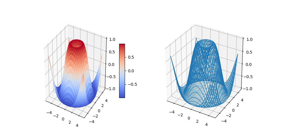 |
Prof. Michela Mapelli lecture diagram: Algorithm flow, spatial treecode, stability region, or HPC parallelization | [[Mathematical_Numerical_Methods_MOC]] |
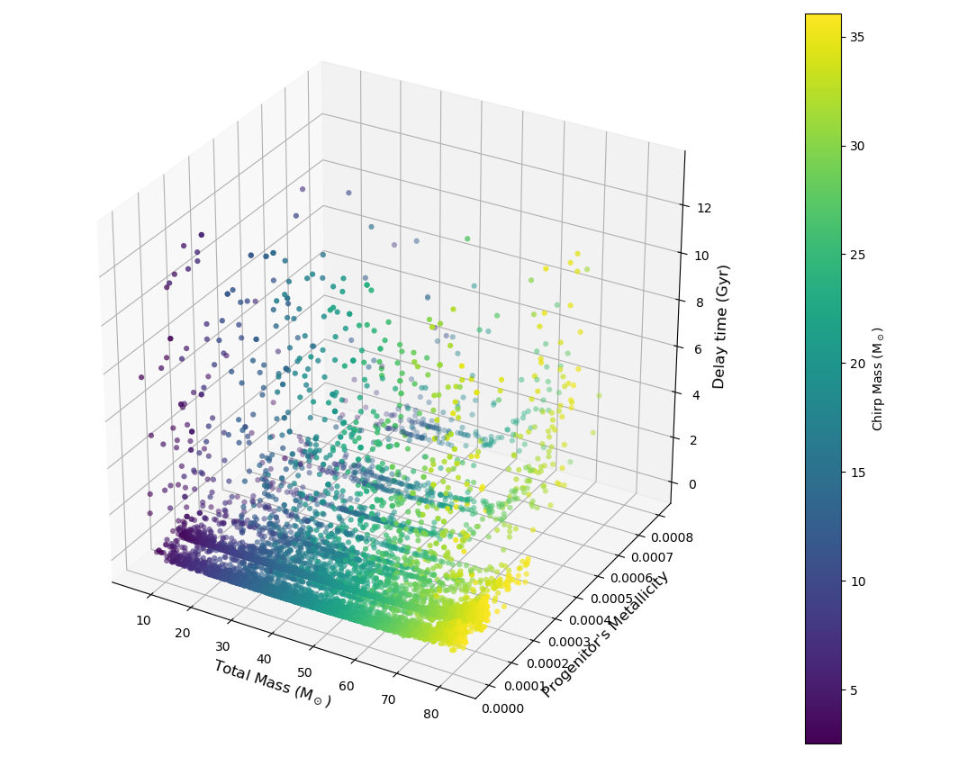 |
Prof. Michela Mapelli lecture diagram: Algorithm flow, spatial treecode, stability region, or HPC parallelization | [[Mathematical_Numerical_Methods_MOC]] |
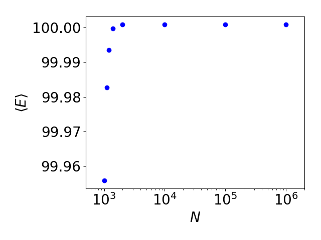 |
Prof. Michela Mapelli lecture diagram: Algorithm flow, spatial treecode, stability region, or HPC parallelization | [[Mathematical_Numerical_Methods_MOC]] |
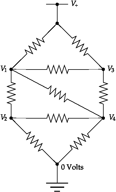 |
Prof. Michela Mapelli lecture diagram: Algorithm flow, spatial treecode, stability region, or HPC parallelization | [[Mathematical_Numerical_Methods_MOC]] |
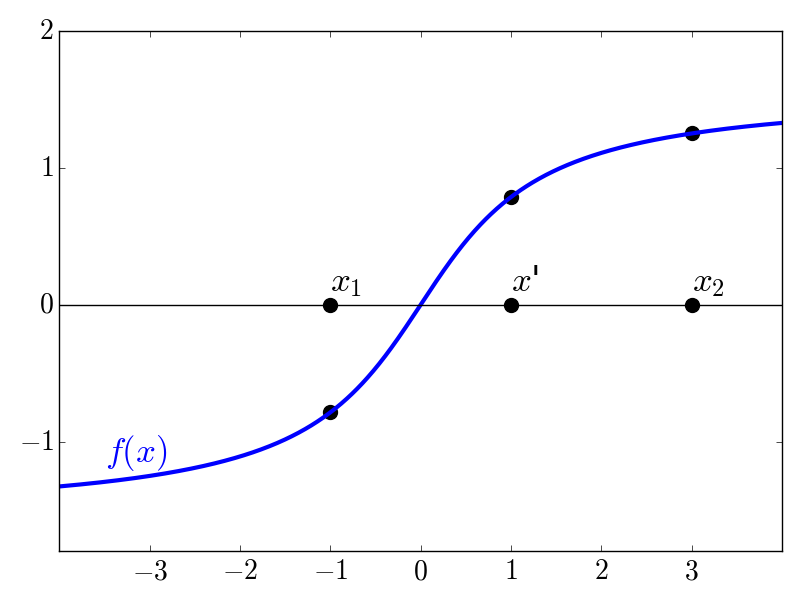 |
Prof. Michela Mapelli lecture diagram: Algorithm flow, spatial treecode, stability region, or HPC parallelization | [[Mathematical_Numerical_Methods_MOC]] |
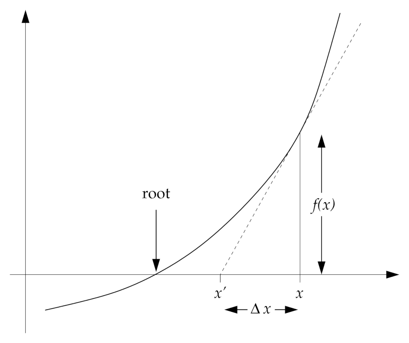 |
Prof. Michela Mapelli lecture diagram: Algorithm flow, spatial treecode, stability region, or HPC parallelization | [[Mathematical_Numerical_Methods_MOC]] |
 |
Prof. Michela Mapelli lecture diagram: Algorithm flow, spatial treecode, stability region, or HPC parallelization | [[Mathematical_Numerical_Methods_MOC]] |
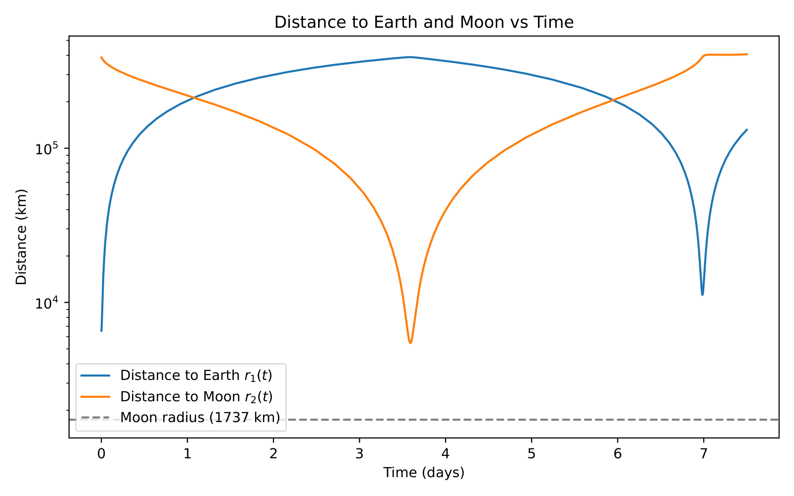 |
Artemis lunar mission simulation in rotating frame / Jacobi integral conservation diagnostic | [[Energy conservation as a diagnostic]] |
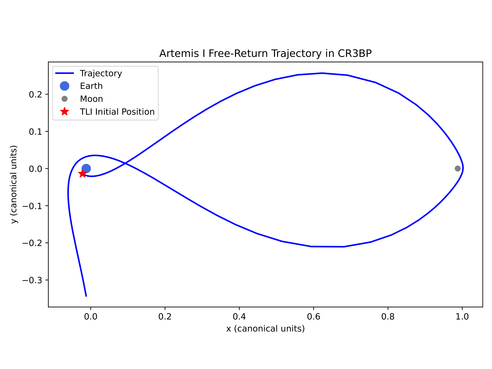 |
Artemis lunar mission simulation in rotating frame / Jacobi integral conservation diagnostic | [[Energy conservation as a diagnostic]] |
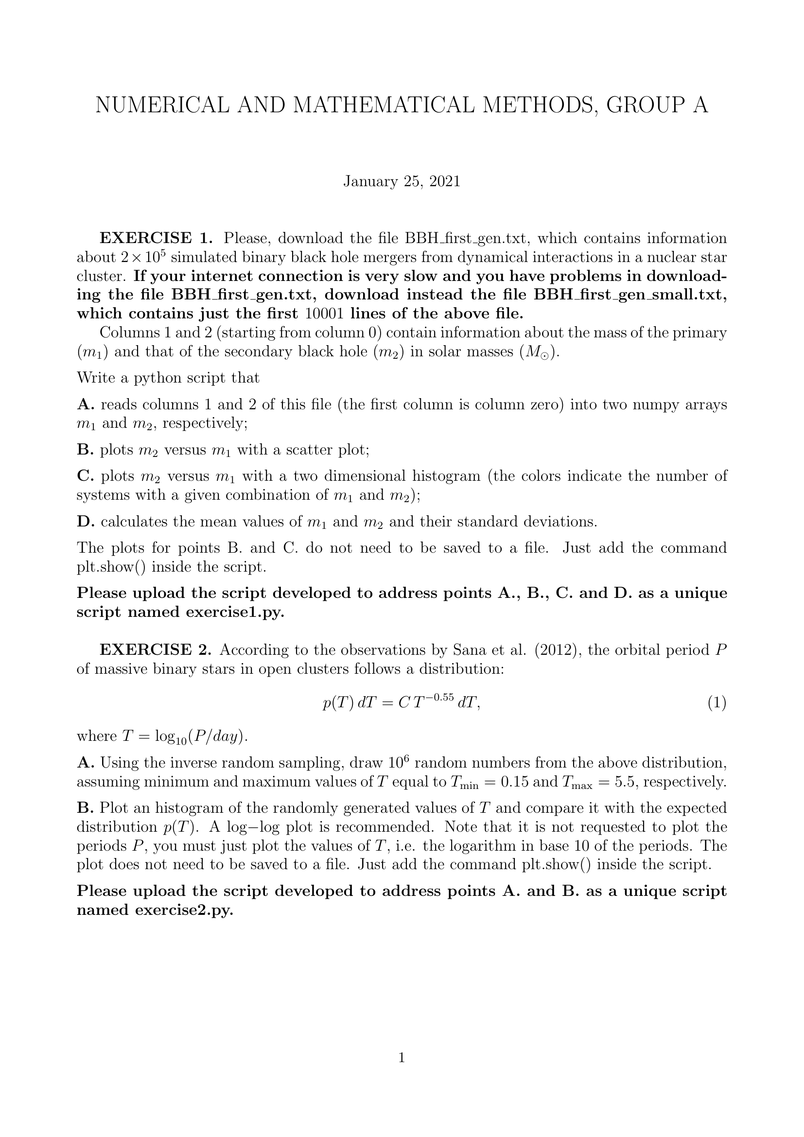 |
Official University of Padua Exam Paper: Numerical ODE integration, stability analysis, and floating-point precision | [[Euler method]] |
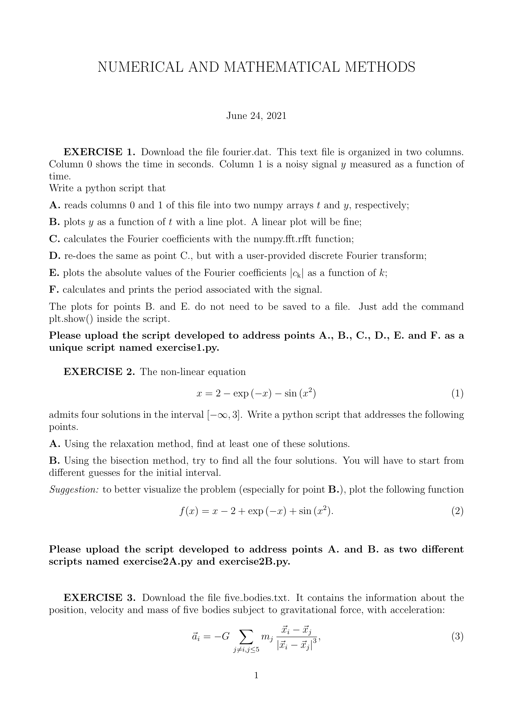 |
Official University of Padua Exam Paper: Numerical ODE integration, stability analysis, and floating-point precision | [[Euler method]] |
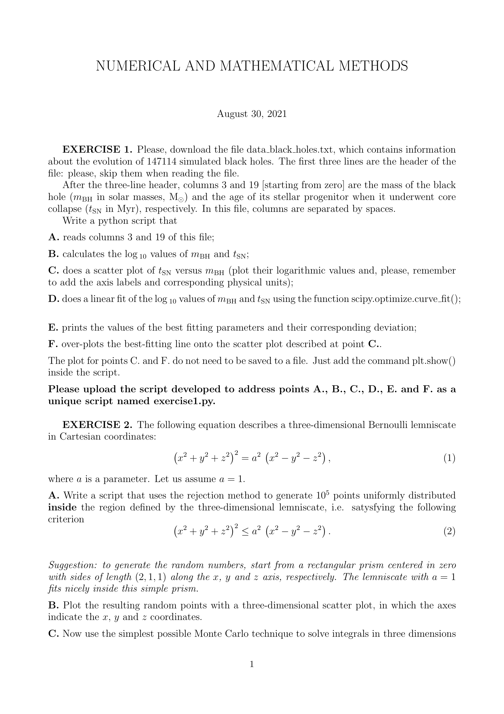 |
Official University of Padua Exam Paper: Numerical ODE integration, stability analysis, and floating-point precision | [[Euler method]] |
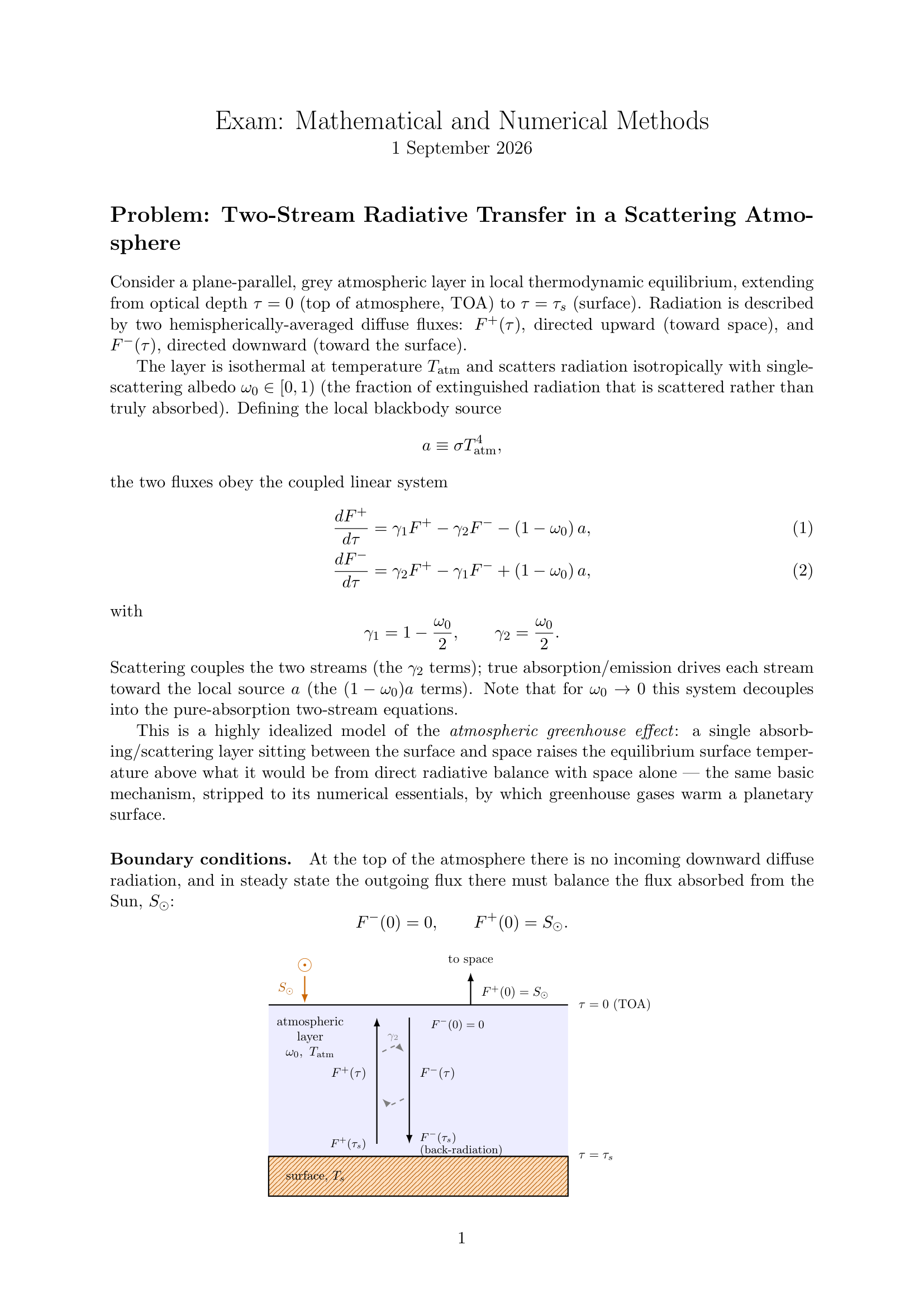 |
Official University of Padua Exam Paper: Numerical ODE integration, stability analysis, and floating-point precision | [[Euler method]] |
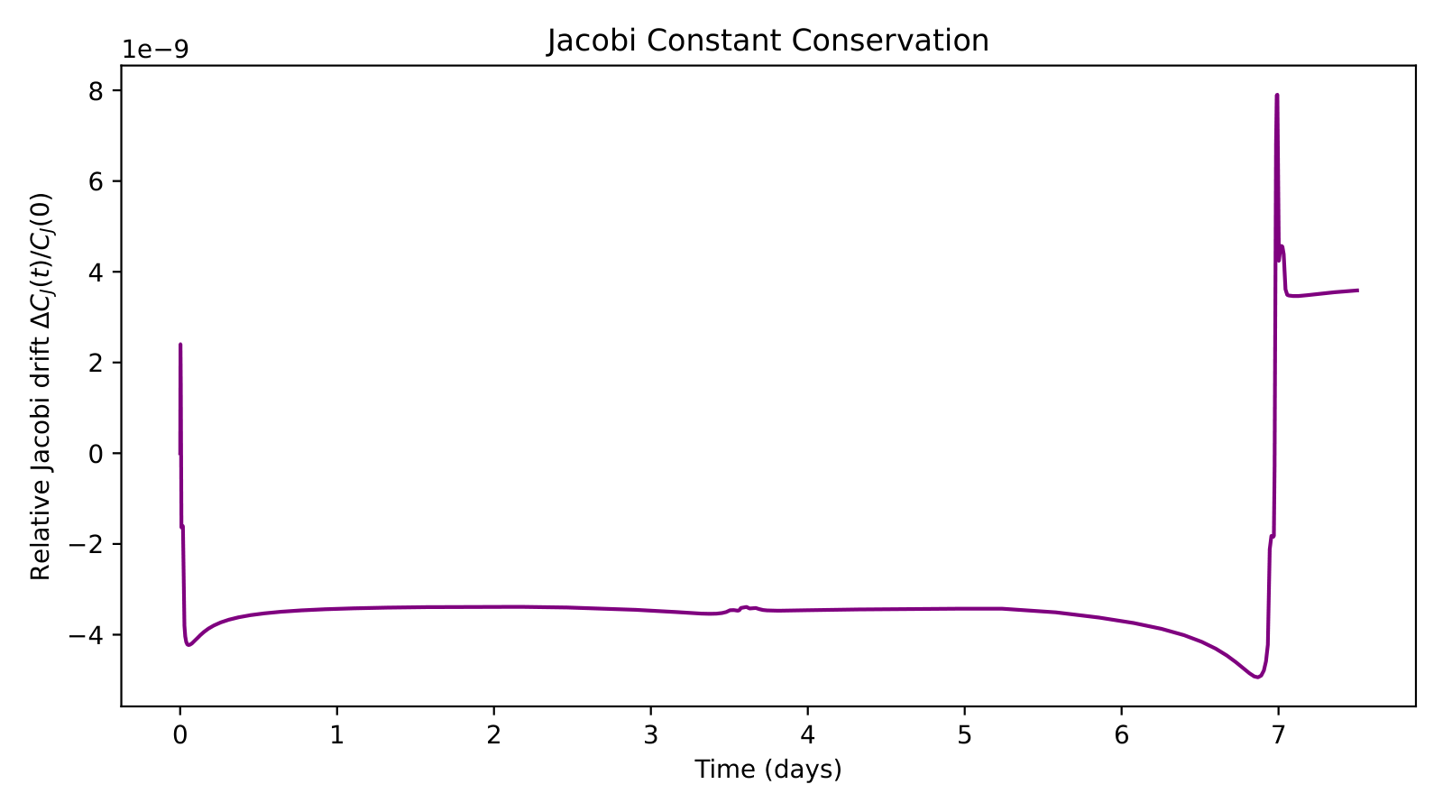 |
Artemis lunar mission simulation in rotating frame / Jacobi integral conservation diagnostic | [[Energy conservation as a diagnostic]] |
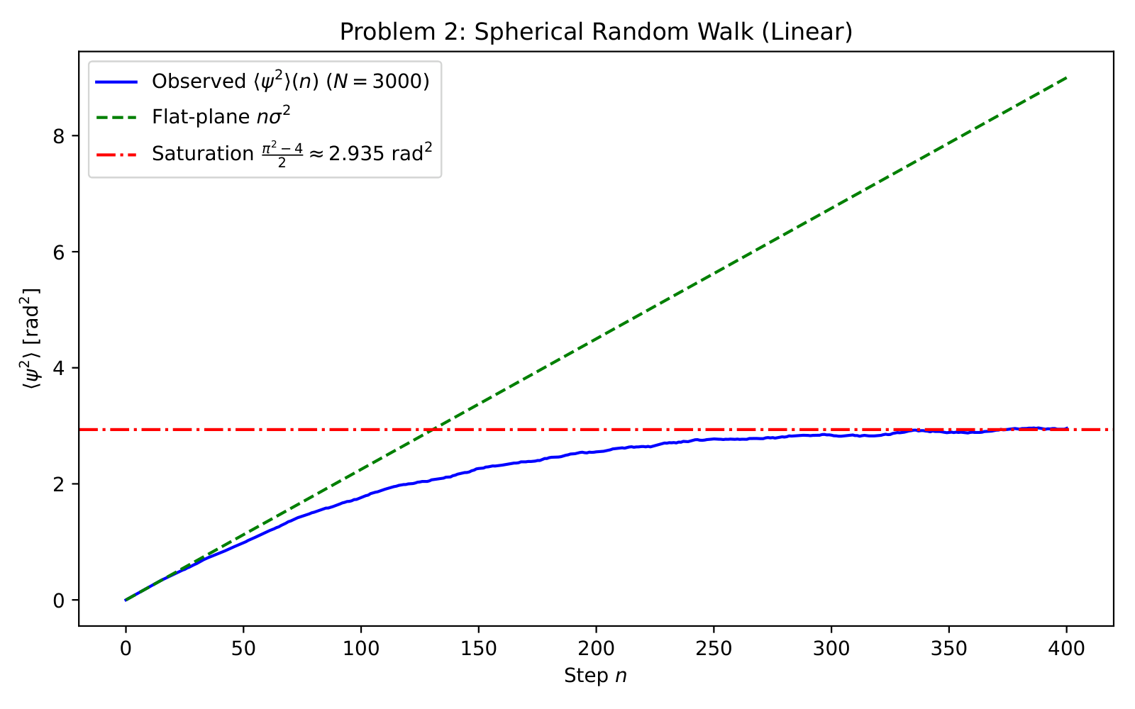 |
Monte Carlo 2D random walk displacement and diffusive scaling law $\sqrt{\langle R^2 \rangle} \propto N^{1/2}$ | [[Box-Muller transform for Gaussian random numbers]] |
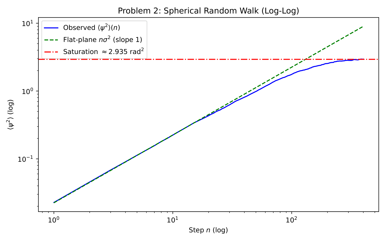 |
Monte Carlo 2D random walk displacement and diffusive scaling law $\sqrt{\langle R^2 \rangle} \propto N^{1/2}$ | [[Box-Muller transform for Gaussian random numbers]] |
 |
Exam Model Answer: Mathematical derivation and Python implementation of Euler, RK4, Leapfrog, and Hermite schemes | [[Leapfrog integrator]] |
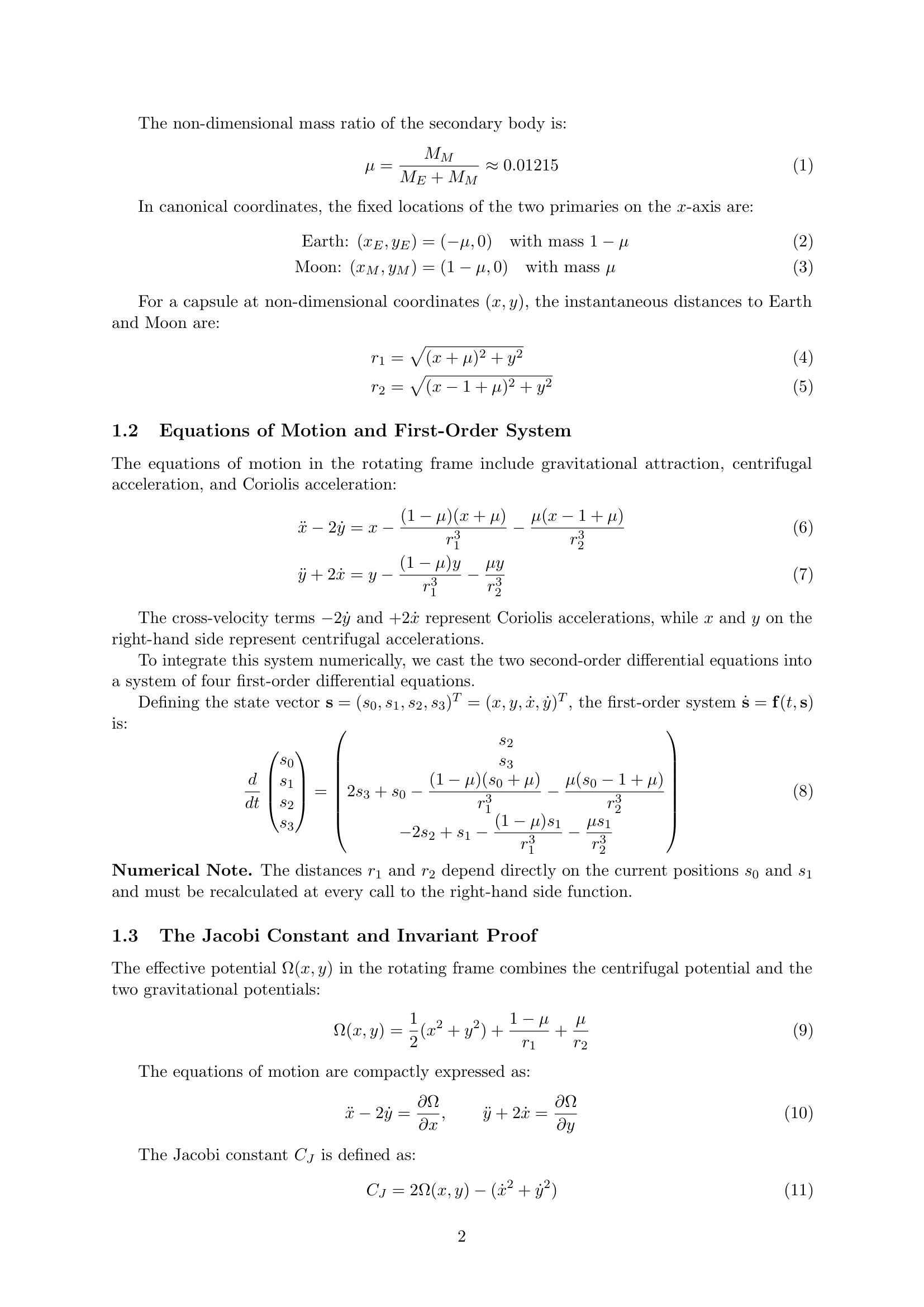 |
Exam Model Answer: Mathematical derivation and Python implementation of Euler, RK4, Leapfrog, and Hermite schemes | [[Leapfrog integrator]] |
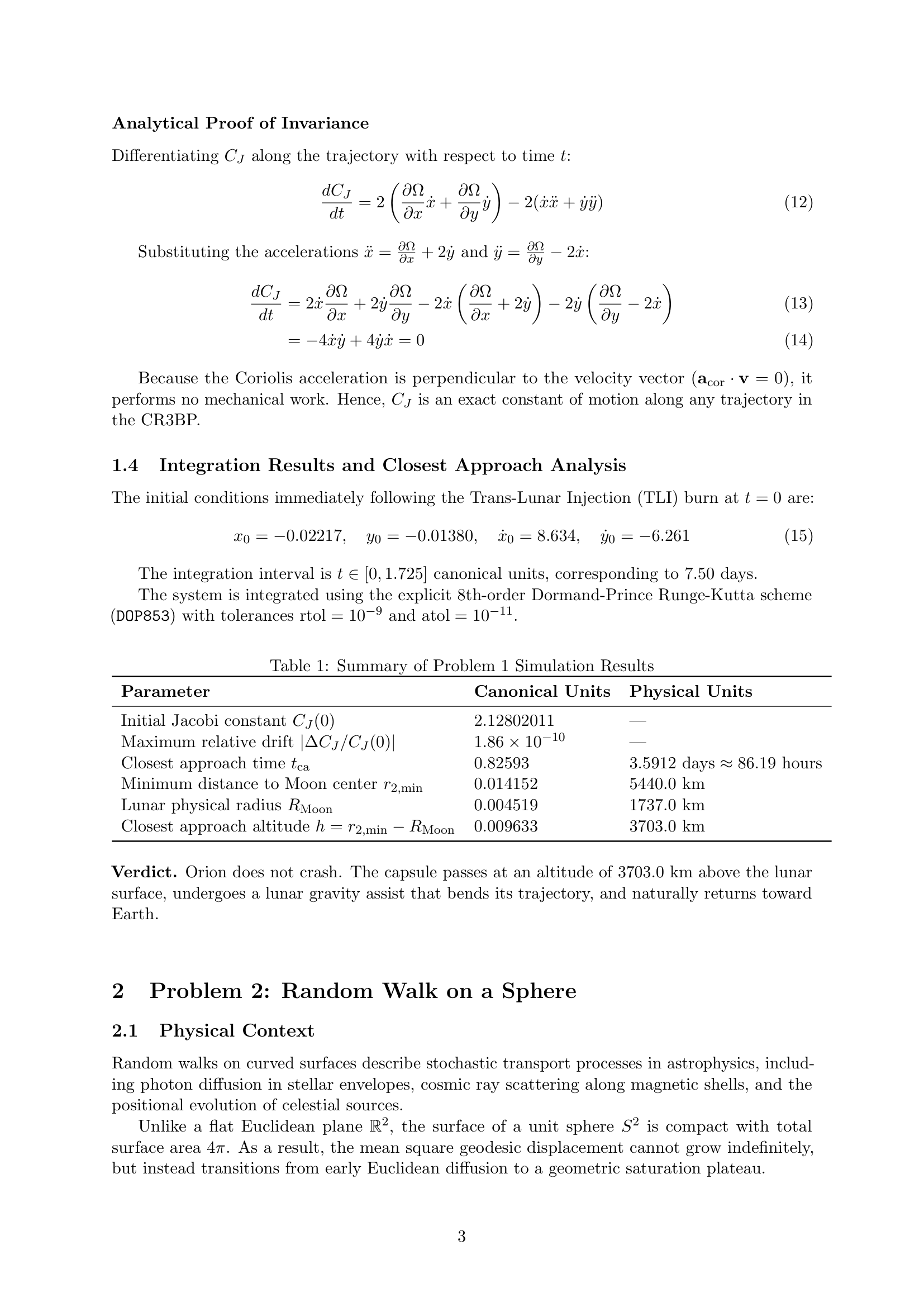 |
Exam Model Answer: Mathematical derivation and Python implementation of Euler, RK4, Leapfrog, and Hermite schemes | [[Leapfrog integrator]] |
 |
Exam Model Answer: Mathematical derivation and Python implementation of Euler, RK4, Leapfrog, and Hermite schemes | [[Leapfrog integrator]] |
Prof. Michela Mapelli Exam & Coding Defense Preparation Matrix
This matrix details the core exam problems, algorithm implementations, and trap points commonly examined by Prof. Michela Mapelli:
Topic 1 - Symplectic Integrators vs Runge-Kutta in Orbital Mechanics
- Blackboard Prompt: Prove why the standard Runge-Kutta 4th order (RK4) method, despite its high accuracy $\mathcal{O}(\Delta t^4)$, is unsuitable for long-term orbital integrations (e.g. planetary orbits or star clusters), whereas the 2nd-order Leapfrog integrator is preferred.
- Starting Equation: \(d\vec{p} \wedge d\vec{q} = {\rm const} \quad \text{(Poincaré symplectic 2-form invariance)}\)
- Derivation & Blackboard Walkthrough:
- Hamiltonian systems preserve phase space volume (Liouville’s theorem) and satisfy the symplectic condition: $M^T J M = J$, where $M = \frac{\partial(\vec{q}{n+1}, \vec{p}{n+1})}{\partial(\vec{q}_n, \vec{p}_n)}$ is the Jacobian of the time-step map and $J = \begin{pmatrix} 0 & I \ -I & 0 \end{pmatrix}$.
- RK4 is a general-purpose non-symplectic integrator. Its Jacobian determinant satisfies $\det(M) \ne 1$. As a consequence, it acts as an artificial dissipation or energy pump, causing a secular (linear in time) drift in orbital energy $\Delta E/E \propto t$.
- Over thousands of dynamical orbits, an RK4 planet will either spiral into the star or escape the system purely due to non-symplectic numerical truncation.
- In contrast, the Leapfrog integrator (Kick-Drift-Kick: $\vec{v}{n+1/2} = \vec{v}_n + \frac{1}{2}\vec{a}_n \Delta t$, $\vec{x}{n+1} = \vec{x}n + \vec{v}{n+1/2} \Delta t$, $\vec{v}{n+1} = \vec{v}{n+1/2} + \frac{1}{2}\vec{a}_{n+1} \Delta t$) is strictly symplectic and time-reversible.
- By backward error analysis, Leapfrog exactly conserves a shadow Hamiltonian $\tilde{H} = H + \mathcal{O}(\Delta t^2)$. Energy errors oscillate within a strictly bounded envelope without secular drift: $\langle \Delta E \rangle = 0$ over millions of orbits!
- Professor Trap Points:
- Trap: Stating that higher order is always better. Higher order non-symplectic methods have smaller errors per step, but the errors accumulate secularly. Symplectic methods preserve invariants of motion globally.
Topic 2 - The Restricted Three-Body Problem & Jacobi Integral
- Blackboard Prompt: Derive the equations of motion for a test mass in the circular restricted three-body problem (CR3BP) in the corotating frame. Prove that the Jacobi integral $C_J$ is an exact constant of motion.
- Derivation & Blackboard Walkthrough:
- In a coordinate frame rotating with constant angular velocity $\vec{\Omega} = \Omega \hat{z}$, the acceleration of a test particle is: \(\ddot{\vec{r}} = -\nabla \Phi_{\rm grav} - 2(\vec{\Omega} \times \dot{\vec{r}}) - \vec{\Omega} \times (\vec{\Omega} \times \vec{r})\)
- Rewrite the centrifugal force as the gradient of a centrifugal potential: $-\vec{\Omega} \times (\vec{\Omega} \times \vec{r}) = \Omega^2(x\hat{x} + y\hat{y}) = -\nabla \Phi_{\rm cent}$, where $\Phi_{\rm cent} = -\frac{1}{2}\Omega^2(x^2 + y^2)$.
- Define the effective potential: $\Phi_{\rm eff} = \Phi_{\rm grav} + \Phi_{\rm cent} = -\frac{G M_1}{r_1} - \frac{G M_2}{r_2} - \frac{1}{2}\Omega^2(x^2 + y^2)$.
- The equation of motion becomes: $\ddot{\vec{r}} + 2(\vec{\Omega} \times \dot{\vec{r}}) = -\nabla \Phi_{\rm eff}$.
- Take the dot product with the velocity vector $\dot{\vec{r}}$: $\dot{\vec{r}} \cdot \ddot{\vec{r}} + 2\dot{\vec{r}} \cdot (\vec{\Omega} \times \dot{\vec{r}}) = -\dot{\vec{r}} \cdot \nabla \Phi_{\rm eff}$.
- The Coriolis term vanishes identically: $\dot{\vec{r}} \cdot (\vec{\Omega} \times \dot{\vec{r}}) = 0$.
- The remaining terms are exact time derivatives: \(\frac{d}{dt}\left(\frac{1}{2}v^2\right) = -\frac{d\Phi_{\rm eff}}{dt} \implies \frac{d}{dt}\left(\frac{1}{2}v^2 + \Phi_{\rm eff}\right) = 0\)
- Multiplying by $-2$, we define the Jacobi Constant: $C_J = -2\Phi_{\rm eff} - v^2 = {\rm const}$.
- Zero-velocity curves ($v=0 \implies C_J = -2\Phi_{\rm eff}$) delineate forbidden regions where $v^2 < 0$, defining the Roche lobes and Lagrange points $L_1$ to $L_5$.
Topic 3 - The Fourth-Order Hermite Predictor-Corrector Scheme
- Blackboard Prompt: Why does Aarseth’s Hermite integrator utilize both acceleration $\vec{a}$ and jerk $\dot{\vec{a}}$? How does it achieve 4th-order accuracy with only one acceleration evaluation per step?
- Derivation & Blackboard Walkthrough:
- In gravitational N-body systems, the jerk $\dot{\vec{a}}_i = \frac{d\vec{a}_i}{dt}$ can be computed analytically at negligible extra cost alongside acceleration: \(\vec{a}_i = \sum_{j \ne i} \frac{G m_j \vec{r}_{ij}}{r_{ij}^3}, \quad \dot{\vec{a}}_i = \sum_{j \ne i} G m_j \left[\frac{\vec{v}_{ij}}{r_{ij}^3} - \frac{3(\vec{r}_{ij} \cdot \vec{v}_{ij})\vec{r}_{ij}}{r_{ij}^5}\right]\)
- Having $\vec{a}n, \dot{\vec{a}}_n$ at $t_n$ and $\vec{a}{n+1}, \dot{\vec{a}}{n+1}$ at $t{n+1}$ provides 4 pieces of information on the derivative, allowing a unique Hermite cubic interpolation polynomial for acceleration.
- Predictor Step (Taylor expansion to 3rd order): \(\vec{x}_{n+1}^p = \vec{x}_n + \vec{v}_n \Delta t + \frac{1}{2}\vec{a}_n \Delta t^2 + \frac{1}{6}\dot{\vec{a}}_n \Delta t^3, \quad \vec{v}_{n+1}^p = \vec{v}_n + \vec{a}_n \Delta t + \frac{1}{2}\dot{\vec{a}}_n \Delta t^2\)
- Evaluate predicted acceleration $\vec{a}{n+1}^p$ and jerk $\dot{\vec{a}}{n+1}^p$ at predicted positions and velocities.
- Higher-derivative extraction: \(\vec{a}_n^{(2)} = \frac{-6(\vec{a}_n - \vec{a}_{n+1}^p) - \Delta t(4\dot{\vec{a}}_n + 2\dot{\vec{a}}_{n+1}^p)}{\Delta t^2}, \quad \vec{a}_n^{(3)} = \frac{12(\vec{a}_n - \vec{a}_{n+1}^p) + 6\Delta t(\dot{\vec{a}}_n + \dot{\vec{a}}_{n+1}^p)}{\Delta t^3}\)
- Corrector Step: \(\vec{x}_{n+1} = \vec{x}_{n+1}^p + \frac{1}{24}\vec{a}_n^{(2)}\Delta t^4 + \frac{1}{120}\vec{a}_n^{(3)}\Delta t^5, \quad \vec{v}_{n+1} = \vec{v}_{n+1}^p + \frac{1}{6}\vec{a}_n^{(2)}\Delta t^3 + \frac{1}{24}\vec{a}_n^{(3)}\Delta t^4\)
- Global error is $\mathcal{O}(\Delta t^4)$, but requires only ONE expensive force evaluation per particle step, compared to 4 evaluations for RK4!
Topic 4 - The Barnes-Hut Tree-Code & Multipole Expansion
- Blackboard Prompt: How does the Barnes-Hut octree algorithm reduce N-body computation from $\mathcal{O}(N^2)$ to $\mathcal{O}(N\log N)$? Explain the multipole acceptance criterion (MAC).
- Derivation & Blackboard Walkthrough:
- Enclose the entire simulation volume in a root cubic cell. Recursively subdivide any cell containing more than 1 particle into 8 octants until each leaf cell contains at most 1 particle. The tree depth is $\mathcal{O}(\log N)$.
- For each node in the tree, compute total mass $M_{\rm cell} = \sum_{k} m_k$ and center of mass $\vec{R}{\rm cm} = \frac{1}{M{\rm cell}}\sum_k m_k \vec{r}_k$.
- When computing force on target particle $i$, traverse tree from root down. At cell $C$ of size $s$ at distance $d = \lvert\vec{r}i - \vec{R}{\rm cm}\rvert$, evaluate the opening angle criterion: \(\theta = \frac{s}{d} < \theta_{\rm crit} \approx 0.5-0.7\)
- If $\theta < \theta_{\rm crit}$, the cell is sufficiently distant: approximate the entire cell as a single monopole gravitational source located at $\vec{R}_{\rm cm}$: \(\vec{a}_i \approx \frac{G M_{\rm cell}(\vec{R}_{\rm cm} - \vec{r}_i)}{\lvert\vec{R}_{\rm cm} - \vec{r}_i\rvert^3}\)
- If $\theta \ge \theta_{\rm crit}$, open the cell and recursively inspect its 8 child octants.
- Traversal requires traversing $\sim \log N$ tree levels for each of the $N$ particles, reducing computational cost from $\mathcal{O}(N^2)$ to $\mathcal{O}(N\log N)$.
Wikipedia and arXiv sources
Every zettel in this map ends with a short sourced section: a definition quoted from Wikipedia (95 zettels) or from the abstract of an arXiv review (0 zettels), and, where a free figure exists, the credited lead figure of the Wikipedia article (Wikimedia Commons) or a figure from an openly licensed arXiv paper. The lecture-slide figures above are unchanged.
| Zettel | Wikipedia | arXiv review | Figure |
|---|---|---|---|
| [[Adaptive step size control]] | Adaptive step size | Commons | |
| [[Adaptive timesteps near close encounters]] | Adaptive step size | Commons | |
| [[Astrophysical N-body problem formulation]] | N-body problem | ||
| [[Bisection method]] | Bisection method | Commons | |
| [[Boundary value PDEs and iteration]] | Boundary value problem | Commons | |
| [[Box-Muller transform for Gaussian random numbers]] | Box–Muller transform | Commons | |
| [[Built-in scipy integrators]] | SciPy | Commons | |
| [[Bulirsch-Stoer extrapolation]] | Bulirsch–Stoer algorithm | ||
| [[Choosing a root finder]] | Root-finding algorithm | Commons | |
| [[Collisional vs collisionless N-body]] | N-body simulation | Commons | |
| [[Computational complexity and speed]] | Computational complexity | ||
| [[Cubic spline interpolation]] | Spline interpolation | ||
| [[Decision tree classifier]] | Decision tree learning | ||
| [[Derivatives of noisy data]] | Numerical differentiation | Commons | |
| [[Discrete Fourier transform]] | Discrete Fourier transform | Commons | |
| [[Energy conservation as a diagnostic]] | Energy drift | Commons | |
| [[Euler method]] | Euler method | Commons | |
| [[Fast Fourier transform algorithm]] | Fast Fourier transform | Commons | |
| [[FFT in scipy and numpy]] | Fast Fourier transform | Commons | |
| [[Finite difference discretization]] | Finite difference method | ||
| [[Fitting practical recipe]] | Curve fitting | Commons | |
| [[Floating point representation and rounding errors]] | Floating-point arithmetic | ||
| [[Forward backward and central differences]] | Finite difference | ||
| [[Fourier series math summary]] | Fourier series | Commons | |
| [[Fourth-order Hermite predictor-corrector]] | Predictor–corrector method | ||
| [[Gauss elimination]] | Gaussian elimination | Commons | |
| [[Gauss-Seidel iteration]] | Gauss–Seidel method | ||
| [[General linear least squares]] | Linear least squares | ||
| [[Goodness of fit and chi-squared]] | Goodness of fit | ||
| [[Gram-Schmidt orthogonalization]] | Gram–Schmidt process | Commons | |
| [[Importance sampling]] | Importance sampling | ||
| [[Initial value PDEs and FTCS]] | FTCS scheme | ||
| [[Initial value vs boundary value problems]] | Boundary value problem | Commons | |
| [[Interpretability vs accuracy in ML]] | Explainable artificial intelligence | ||
| [[Inverse transform sampling]] | Inverse transform sampling | Commons | |
| [[Iris dataset and the ML hello world]] | Iris flower data set | Commons | |
| [[Lagrange polynomial interpolation]] | Lagrange polynomial | Commons | |
| [[Leapfrog integrator]] | Leapfrog integration | ||
| [[Linear interpolation]] | Linear interpolation | Commons | |
| [[Linear least squares]] | Linear least squares | ||
| [[Linux for the astrophysicist]] | Linux | ||
| [[LU decomposition]] | LU decomposition | ||
| [[Matplotlib plotting essentials]] | Matplotlib | ||
| [[Matrix diagonalization $A = VDV^T$]] | Diagonalizable matrix | ||
| [[Matrix inverse via linear systems]] | Invertible matrix | ||
| [[Modified midpoint method]] | Midpoint method | Commons | |
| [[Monte Carlo integration mean value method]] | Monte Carlo integration | Commons | |
| [[Multidimensional Monte Carlo integration]] | Monte Carlo integration | Commons | |
| [[N-body with Euler vs midpoint vs leapfrog]] | N-body simulation | Commons | |
| [[Newton divided differences]] | Newton polynomial | ||
| [[Newton-Raphson for systems of equations]] | Newton’s method | Commons | |
| [[Newton-Raphson method]] | Newton’s method | Commons | |
| [[Non-linear fitting with scipy]] | Non-linear least squares | ||
| [[Numerical problem solving workflow]] | Numerical analysis | ||
| [[Numpy arrays vs Python lists]] | NumPy | Commons | |
| [[Optimal step size for derivatives]] | Numerical differentiation | Commons | |
| [[Overrelaxation]] | Successive over-relaxation | ||
| [[Pandas for tabular astrophysics data]] | Pandas (software) | ||
| [[Partial numerical derivatives]] | Numerical differentiation | Commons | |
| [[Partial pivoting]] | Pivot element | ||
| [[Physical interpretation of the FFT]] | Fast Fourier transform | Commons | |
| [[Polynomial fitting]] | Polynomial regression | Commons | |
| [[Power iteration]] | Power iteration | ||
| [[Power spectrum estimation]] | Spectral density estimation | ||
| [[Pros and cons of linear solvers]] | System of linear equations | ||
| [[Pseudo-random number generators]] | Pseudorandom number generator | ||
| [[Python language essentials]] | Python (programming language) | ||
| [[QR algorithm for eigenvalues]] | QR algorithm | ||
| [[QR decomposition]] | QR decomposition | ||
| [[Random number seeds]] | Random seed | ||
| [[Rejection sampling]] | Rejection sampling | Commons | |
| [[Relaxation method]] | Relaxation (iterative method) | ||
| [[Roundoff vs truncation balance]] | Round-off error | ||
| [[Runge phenomenon]] | Runge’s phenomenon | Commons | |
| [[Runge-Kutta 2 midpoint method]] | Midpoint method | Commons | |
| [[Runge-Kutta 4 method]] | Runge–Kutta methods | Commons | |
| [[Scipy and astropy quick reference]] | SciPy | Commons | |
| [[Scipy interpolation tools]] | Interpolation | ||
| [[Second derivatives]] | Numerical differentiation | Commons | |
| [[Shooting method]] | Shooting method | ||
| [[Simpson’s rule]] | Simpson’s rule | Commons | |
| [[Sorting algorithms overview]] | Sorting algorithm | Commons | |
| [[Stability and the Courant condition]] | Courant–Friedrichs–Lewy condition | ||
| [[Systems of ODEs and higher-order ODEs]] | Ordinary differential equation | Commons | |
| [[The conda environment]] | Conda (package manager) | ||
| [[The Pythagorean three-body problem]] | Three-body problem | Commons | |
| [[Trapezoidal rule error estimate]] | Trapezoidal rule | Commons | |
| [[Trapezoidal rule]] | Trapezoidal rule | Commons | |
| [[Truncation error and order of accuracy]] | Truncation error | ||
| [[Two-dimensional interpolation]] | Bilinear interpolation | Commons | |
| [[Vectorization and python speed]] | Array programming | ||
| [[Verifying random samples]] | Kolmogorov–Smirnov test | Commons | |
| [[Weighted least squares]] | Weighted least squares | ||
| [[What is machine learning]] | Machine learning | ||
| [[When to use implicit schemes]] | Explicit and implicit methods |
Essential Mathematical & Numerical Methods Formulas Quick Sheet
| Method / Law | Mathematical Expression | Order & Computational Complexity | ||||
|---|---|---|---|---|---|---|
| Forward Euler | $x_{n+1} = x_n + f(x_n, t_n)\Delta t$ | $\mathcal{O}(\Delta t)$ global error, unconditionally unstable for oscillations | ||||
| Leapfrog (KDK) | $\vec{v}{n+1/2} = \vec{v}_n + \frac{\Delta t}{2}\vec{a}_n, \; \vec{x}{n+1} = \vec{x}n + \Delta t\vec{v}{n+1/2}, \; \vec{v}{n+1} = \vec{v}{n+1/2} + \frac{\Delta t}{2}\vec{a}_{n+1}$ | $\mathcal{O}(\Delta t^2)$ global error, symplectic and time-reversible | ||||
| Runge-Kutta 4 (RK4) | $x_{n+1} = x_n + \frac{\Delta t}{6}(k_1 + 2k_2 + 2k_3 + k_4)$ | $\mathcal{O}(\Delta t^4)$ global error, 4 force evaluations per step | ||||
| Hermite 4th Order | $\vec{x}_{n+1} = \vec{x}^p + \frac{\Delta t^4}{24}\vec{a}^{(2)} + \frac{\Delta t^5}{120}\vec{a}^{(3)}$ | $\mathcal{O}(\Delta t^4)$ global error, uses analytical jerk $\dot{\vec{a}}$ | ||||
| Plummer Softened Force | $\vec{F}{ij} = -\frac{G m_i m_j (\vec{r}_i - \vec{r}_j)}{(r{ij}^2 + \epsilon^2)^{3/2}}$ | Eliminates singularity at $r_{ij} \to 0$, introduces core radius $\epsilon$ | ||||
| Jacobi Constant | $C_J = -2\Phi_{\rm eff} - v^2 = \Omega^2(x^2 + y^2) + 2\frac{GM_1}{r_1} + 2\frac{GM_2}{r_2} - v^2$ | Exact invariant in circular restricted 3-body problem (CR3BP) | ||||
| Random Walk RMS Spread | $\sqrt{\langle R^2(N) \rangle} = l_{\rm step} \sqrt{N}$ | Standard diffusive scaling in $D$ dimensions | ||||
| Barnes-Hut MAC | $\theta = \frac{s}{d} < \theta_{\rm crit} \approx 0.5-0.7$ | $\mathcal{O}(N\log N)$ N-body treecode multipole acceptance condition | ||||
| Newton-Raphson Iteration | $x_{n+1} = x_n - \frac{f(x_n)}{f’(x_n)}$ | Quadratic local convergence $ | e_{n+1} | \propto | e_n | ^2$ |
| CFL Stability Condition | $C = \frac{u \Delta t}{\Delta x} \le C_{\rm max} = 1$ | Courant condition for explicit hyperbolic PDE stability | ||||
| Metropolis Acceptance Ratio | $\alpha = \min\left(1, \frac{P(x’)}{P(x)}\frac{q(x | x’)}{q(x’ | x)}\right)$ | MCMC transition probability preserving detailed balance |
Follow along on Instagram @your.astrophysicist · Report an issue