Lab_High-Energy_MOC
High Energy Astrophysics Laboratory - Map of Content
A.Y. 2025/2026, Prof. Stefano Ciroi, University of Padova.
The central thread of this course is a single question:
- how do we detect, measure, and interpret radiation from the most violent objects in the universe?
Every topic connects to this chain: \(\text{violent source} \to \text{photons} \to \text{atmosphere blocks them} \to \text{space telescope} \to \text{detector} \to \text{counts} \to \text{spectrum} \to \text{physics}\)
All notes are linked below. The detailed derivations, equations, and figures live in each individual note.
Block 1 - Introduction and Observational Basics
Why X-ray astronomy must be done from space, and what “measuring” a source actually means.
- Introduction of High Energy Instrumentation - course overview and motivation
- [[Atmospheric transmission]] - the four atmospheric effects, X-ray opacity, space as the only solution
- [[Seeing Effect]] - Kolmogorov turbulence, Fried parameter, seeing disk, adaptive optics
- [[Luminosity and Flux for -Instrumentations]] - $F = L/4\pi d_L^2$, photon flux, count rate, absorption, K-correction, ECF, hardness ratio
- [[Luminosity]] - quick reference, typical values
- [[Telescope resolving power]] - Rayleigh criterion, plate scale, limiting factors by telescope type
- [[Rayleigh criterion]] - Airy disk derivation, $\theta = 1.22\lambda/D$, examples
- [[Point Spread Function (PSF)]] - PSF definition, FWHM vs HPD, EEF, on-axis vs off-axis
- [[A Brief History of X-ray and Gamma-ray Missions]] - from Giacconi 1962 to eROSITA 2019
Block 2 - X-ray Focusing Telescopes
How we build telescopes that reflect X-rays.
- [[Grazing incidence]] - refractive index $n = 1-\delta+i\beta$, critical angle $\theta_c \approx \sqrt{2\delta} \propto \sqrt{\rho}/E$, high-Z coatings
- [[Bragg Reflection]] - multilayer coatings, modified Bragg equation, NuSTAR, hard X-ray focusing
- [[Wolter Telescope]] - Wolter I/II/III, Abbe sine condition, two reflections, nested shells
- [[Effective Area]] - $A_{eff} = A_{geo} \times R_{mirrors} \times QE \times T_{filter}$, energy dependence, mission comparison
- [[Angular Resolution]] - HPD definition, blur circle sources ($\sigma_{diff}^2 + \sigma_{geom}^2 + \sigma_{rough}^2 + \sigma_{align}^2$), mission comparison
Block 3 - Alternative Instruments (Hard X-ray and Gamma-ray)
What to use when you cannot focus.
- [[Processes of photon-matter interaction]] - three processes, linear attenuation coefficient $\mu = \sigma n$, mean free path $\lambda = 1/\mu$, domain diagram
- [[Photoelectric absorption]] - $\sigma_{ph} \propto Z^{4-5}/E^3$, absorption edges, relation to $\beta$, ISM column density
- [[Compton scattering and pair production]] - Compton formula $E’_{ph}$, Klein-Nishina, pair production threshold $1.022~\text{MeV}$, annihilation
- [[Mechanical Collimator]] - $\Delta\theta = d/L$, on/off method, no imaging, source confusion
- [[Coded Mask]] - shadowgram $D = S \otimes M + B$, deconvolution, $S’ = S + B \otimes G$, INTEGRAL IBIS, Swift BAT
- [[Compton Telescope]] - two planes (scatterer + absorber), source cone, time-of-flight rejection, COMPTEL/CGRO
Block 4 - Detectors - CCDs
How X-ray photons become electrons and counts.
- [[Charge-Coupled Device]] - semiconductors, energy bands, doping, n-type and p-type silicon
- [[The p-n junction]] - diffusion, depletion region, reverse bias, buried channel
- [[CCD readout]] - MOS capacitor, 3-phase clocking, serial register, readout noise $\sigma_{RON}$, CTE
- [[CCDs for X-rays]] - $N_e = E_{ph}/w$ ($w = 3.68~\text{eV}$), photon counting mode, grades, pile-up, energy resolution
- [[Quantum efficiency]] - transmission through dead layers $T = e^{-\mu t}$, absorption in depletion $A = 1 - e^{-\mu_{Si}d}$, front vs back illumination, optical blocking filter
Block 5 - X-ray Gratings
High-resolution spectroscopy with dispersive elements.
- [[X-ray diffraction grating]] - transmission: $d(\sin\theta - \sin i) = m\lambda$, reflection: $d(\cos\theta - \cos i) = m\lambda$, Rowland circle, Chandra HETGS, XMM-Newton RGS
- [[Appendix D - Gratings and spectrographs]] - grating equation geometry, blazed gratings, angular dispersion, resolving power $R = mN$
Block 6 - Astrostatistics
How to go from counts to meaningful physics.
- [[Astrostatistics]] - introduction, the full chain from photons to physics
- [[Distributions]] - probability distributions, Poisson $f(k;\lambda) = \lambda^k e^{-\lambda}/k!$, $E[k] = V[k] = \lambda$, Gaussian approximation
- [[Signal-Noise Ratio]] - $SNR = st/\sqrt{(s+b)t}$, source-dominated vs background-dominated, why angular resolution matters
- [[Fitting]] - $\chi^2$, reduced $\chi^2$, degrees of freedom, C-statistics (Kaastra 2017), forward folding, RMF, ARF
- [[p-value]] - definition, null hypothesis, 4-step hypothesis test, critical warning
Block 7 - Radiative Processes
The physics of what produces X-ray and gamma-ray emission.
- [[Radiative Processes]] - Larmor formula, three mechanisms overview, particle distributions
- [[Bremsstrahlung]] - thermal free-free emission, flat spectrum + exponential cutoff at $h\nu \sim k_BT$, galaxy clusters, emission measure
- [[Synchroton]] - relativistic electrons in $B$, $\nu_c \propto \gamma^2 qB/m_ec$, power-law spectrum $f_\nu \propto \nu^{-\alpha}$ with $\alpha = (s-1)/2$, cooling break
- [[Compton and Inverse Compton]] - Thomson/Compton, Klein-Nishina, IC energy boost $E_f \approx \gamma^2 E_i$, $P_{IC}/P_{syn} = U_{ph}/U_B$, Comptonization, y-parameter
Block 8 - Accretion onto Compact Objects
The extreme sources we observe.
- [[Accretion onto compact objects]] - $L_{acc} = \eta\dot{m}c^2$, $L_{Edd} \approx 1.3\times10^{38}(M/M_\odot)$ erg/s, $T(r) \propto r^{-3/4}$, ISCO, XRBs, AGN unified model
- [[Kerr Metric Horizon and Ergosphere Geometry]] - horizon radii $r_\pm$, ergosphere $r_{\rm ergo}(\theta)$, ZAMO/horizon angular velocity $\Omega_H$
- [[Innermost Stable Circular Orbit ISCO]] - spin-dependent $r_{\rm ISCO}(a_)$, accretion radiative efficiency $\eta(a_)$ from $0.057$ to $0.42$
- [[Blandford-Znajek Mechanism]] - spin-powered jet extraction, $P_{BZ}=\frac{\kappa}{4\pi c}\Phi_H^2\Omega_H^2$, membrane paradigm
- [[Relativistic Iron Line Profiles]] - disk-line redshift factor $g(r,\phi,i)$, double-horned profile, spin diagnostics via the red wing
Literature & Primary Sources
Canonical and modern arXiv astro-ph.HE benchmark papers underlying the accretion, jet, and reverberation physics above.
- [[Shakura_Sunyaev_1973_Thin_Accretion_Disk_Theory|Shakura & Sunyaev (1973) - Black Holes in Binary Systems]] - $\alpha$-disk theory, $T(r)\propto r^{-3/4}$ derivation
- [[Blandford_Znajek_1977_Electromagnetic_Extraction_Kerr_BH|Blandford & Znajek (1977) - Electromagnetic Extraction from Kerr Black Holes]] - spin-powered jet mechanism, membrane paradigm
- [[Fabian_2009_Broad_Iron_Line_Reverberation_1H0707-495|Fabian et al. (2009) - Broad Iron Line Reverberation in 1H0707-495]] - X-ray reverberation lag, compact corona geometry
- [[Blandford_Meier_Readhead_2019_Relativistic_AGN_Jets|Blandford, Meier & Readhead (2019) - Relativistic Jets from Active Galactic Nuclei]] - unified jet-launching review, MAD state, blazar beaming
Appendices (background material)
- [[Appendix A - Optical telescopes]] - aperture ratio, plate scale, conic sections
- [[Appendix B - Aberrations]] - Seidel theory, spherical aberration, coma
- [[Appendix C - Telescope configurations]] - Newton, Cassegrain, Ritchey-Chrétien
- [[Appendix E - Astronomical coordinates]] - altazimuth, equatorial, vernal equinox, precession, J2000
Oral Exam Questions and Answers
Block 1 - Introduction and Observational Basics
Q1. Why is it impossible to do X-ray astronomy from the ground? What is the physical process responsible?
X-ray photons with energies above $\sim 0.1~\text{keV}$ are absorbed by the Earth’s atmosphere through photoelectric absorption. The atmospheric atoms (N, O, Ar) have ionization energies in this range. The cross-section goes as $\sigma_{ph} \propto Z^{4-5}/E^3$, so lower energies are more strongly absorbed. The optical depth $\tau_{atm} \gg 1$ at all X-ray energies below $\sim 100$ keV. The atmospheric hydrogen column density is $N_H^{atm} \sim 10^{25}$ cm$^{-2}$, which absorbs everything below $\sim 100$ keV completely. Therefore all X-ray observatories must be satellites.
Q2. Define flux and luminosity. Write the relation between them and state all assumptions.
Luminosity $L$ is the total power emitted by a source, intrinsic and independent of the observer. Flux $F$ is the power received per unit collecting area at the detector.
For an isotropic point source at luminosity distance $d_L$: \(F = \frac{L}{4\pi d_L^2}\)
Assumptions: (1) isotropic emission. (2) transparent medium (no absorption). (3) unresolved source. (4) for cosmological distances, $d_L = (1+z)d_C$ and the K-correction $K(z) = (1+z)^{2-\Gamma}$ must be applied for the observed vs rest-frame band.
Q3. What is a photon flux and why is it used in X-ray astronomy instead of energy flux?
The photon flux $\mathcal{F}(E) = F_E/E$ [ph/s/cm²/keV] counts photons per unit energy, not energy per unit energy. It is used because X-ray detectors (CCDs, proportional counters) count individual photons, each photon arrives as a discrete event and its deposited charge is proportional to its energy. Spectral fitting software (XSPEC, Sherpa) models the photon spectrum, folds it through the instrument response, and compares predicted counts to observed counts. Working in photon units avoids implicit spectral-shape assumptions needed to convert count rates to energy flux.
Q4. What is the Rayleigh criterion? What actually limits X-ray telescope resolution?
The Rayleigh criterion states two point sources are just resolved when the central maximum of one’s Airy disk coincides with the first minimum of the other’s: $\theta_{min} = 1.22\lambda/D$.
For X-ray telescopes, diffraction is completely irrelevant, at 1 keV with a 1-m aperture, $\theta_{diff} \approx 0.0003’’$. The actual resolution is characterized by HPD and is dominated by: \(\sigma_{blur}^2 = \sigma_{diff}^2 + \sigma_{geom}^2 + \sigma_{rough}^2 + \sigma_{align}^2\) where mirror figure errors, surface roughness, and alignment errors all contribute. Chandra has HPD $\approx 0.5’’$. XMM-Newton has HPD $\approx 14’’$.
Block 2 - X-ray Telescopes
Q5. Derive the critical angle for total external reflection of X-rays. Why does it depend on energy?
The refractive index of the mirror material is $n = 1 - \delta + i\beta$ with $\delta > 0$, so $n < 1$. Applying Snell’s law for grazing angle $\theta_c$ (measured from the surface): \(\cos\theta_c = n \approx 1 - \delta\)
Using the small-angle approximation $\cos\theta_c \approx 1 - \theta_c^2/2$: \(\theta_c \approx \sqrt{2\delta}\)
Since $\delta \propto \rho f_1 \lambda^2/W_m \propto \rho/E^2$ (at high energies): \(\theta_c \propto \frac{\sqrt{\rho}}{E}\)
The critical angle decreases with energy → higher-energy photons require shallower grazing angles → above the cutoff energy for a given angle, the mirror stops reflecting → sharp drop in $A_{eff}(E)$.
Q6. Describe the Wolter Type I telescope. Why are two reflections needed?
A Wolter I telescope uses a paraboloid mirror followed by a hyperboloid mirror, both confocal, both at grazing incidence.
Two reflections are needed to satisfy the Abbe sine condition: \(\frac{h}{\sin\theta} = R = \text{const}\)
A single paraboloid perfectly focuses on-axis sources but produces severe coma for off-axis sources, the useful field of view is negligibly small. The second reflection in the Wolter geometry ensures the same optical path for all rays, eliminating coma and producing a usable field of view. The factor $R^2(E)$ in $A_{eff}$ comes from two successive reflections with reflectivity $R(E)$ each.
Q7. Write the effective area formula and explain each term. What limits it at low and high energies?
\[A_{eff}(E) = A_{geo} \times R_{mirrors}(E) \times QE(E) \times T_{filter}(E)\]- $A_{geo}$: annular geometric area of the mirror shell(s), nested shells add their contributions
- $R_{mirrors}(E)$: grazing-incidence reflectivity - falls sharply above the energy where $\theta_c(E) < \theta_{graze}$
- $QE(E)$: quantum efficiency - absorption in dead layers limits low E, finite depletion depth limits high E
- $T_{filter}(E)$: optical blocking filter - absorbs soft X-rays below $\sim 0.3$ keV
Low-energy limit: dead layers + filter absorb soft photons High-energy limit: $\theta_c \propto 1/E$ → reflectivity falls → use Bragg multilayers (NuSTAR) to extend beyond 10 keV
Q8. Explain the coded mask principle. Write the deconvolution equation and explain the background residual.
A coded mask has open and closed pixels in a pseudo-random pattern. X-ray sources cast the mask shadow onto the detector, the shadowgram $D$ is a convolution: \(D = S \otimes M + B\)
To recover the sky $S$, find a decoding array $G$ such that $M \otimes G = \delta$: \(S' = D \otimes G = S + B \otimes G\)
The term $B \otimes G$ is the background convolved with the decoding function. It must be estimated and subtracted. Non-uniform or variable background introduces systematic residuals in the reconstructed image. Angular resolution: $\theta \sim d_{pixel}/D_{det}$ (mask pixel size / detector-mask distance).
Block 3 - Detectors (CCDs)
Q9. How does a CCD detect an X-ray photon? How does this differ from optical detection?
An X-ray photon absorbed in the silicon depletion region creates $N_e = E_{ph}/w$ electron-hole pairs, where $w = 3.68$ eV. The charge is proportional to the photon energy, both position (which pixel) and energy (how much charge) are measured simultaneously.
For optical photons ($E_{ph} \sim 2$ to $3$ eV): at most $N_e = 1$, no energy information. Optical CCDs integrate many photons. X-ray CCDs must operate in photon counting mode (at most 1 photon per pixel per frame), so each event gives an independent energy measurement.
Q10. What is pile-up? When does it occur and what are its effects?
Pile-up occurs when two or more photons arrive in the same pixel within one readout frame. Their charges sum, and the detector records a single event with the combined energy.
Effects:
- Spectral hardening: summed energy mimics a harder photon - spectrum appears harder than it is
- Count rate saturation: multiple photons counted as one → flux underestimated
- Grade migration: charge cloud shape changes → events misclassified or rejected
Pile-up probability: $p \approx 1 - e^{-f \cdot t_{frame}}$. Mitigation: smaller CCD sub-window (shorter frame time), grating spectroscopy for bright sources.
Q11. Derive the energy resolution formula. What is the Fano factor?
If $N_e = E_{ph}/w$ electrons are created on average, naively $\sigma^2 = N_e$ (Poisson). But ionization events are correlated, energy is shared among all created pairs (energy conservation). This reduces fluctuations by the Fano factor $F = 0.115$ for silicon: \(\sigma^2(N_e) = F \cdot N_e = F \cdot E_{ph}/w\)
Adding readout noise $\sigma_{RON}$ in quadrature and converting to energy (1 $e^-$ = $w$ eV): \(\text{FWHM} = 2.35 \cdot w \cdot \sqrt{\sigma_{RON}^2 + F \cdot E_{ph}/w}\)
For Fe K$\alpha$ at 6.4 keV with $\sigma_{RON} = 5$ $e^-$: FWHM $\approx 150$ eV, so $R = E/\Delta E \approx 43$.
Block 4 - Astrostatistics
Q12. Why does Poisson statistics apply in X-ray astronomy? Derive the mean and variance.
X-ray photons arrive as independent, rare events from a steady source, the number of photons in time $t$ satisfies: (1) independence, (2) constant rate $\lambda$, (3) at most one event per infinitesimal interval. This defines a Poisson process: $f(k;\lambda) = \lambda^k e^{-\lambda}/k!$
Mean: $E[k] = \lambda$ (by direct calculation, shifting the summation index)
Variance: $V[k] = E[k^2] - \lambda^2 = \lambda^2 + \lambda - \lambda^2 = \lambda$
Both equal $\lambda$: noise $\sigma = \sqrt{\lambda}$, relative noise $= 1/\sqrt{\lambda}$, faint sources have large fractional uncertainty.
Q13. Derive the SNR formula. When does it not grow as $\sqrt{t}$?
Source counts $N_{src} = st$, background counts $N_{bg} = bt$. Total detected counts $(s+b)t$ with Poisson noise $\sqrt{(s+b)t}$. The source signal over noise: \(SNR = \frac{st}{\sqrt{(s+b)t}} = \frac{s\sqrt{t}}{\sqrt{s+b}}\)
$SNR \propto \sqrt{t}$ in both limiting regimes (source- and background-dominated). It stops growing as $\sqrt{t}$ when systematics dominate: imperfect background subtraction, calibration uncertainty, confusion with nearby sources. these create irreducible floors that more exposure cannot overcome.
Q14. When should you use C-statistics instead of $\chi^2$?
$\chi^2$ requires Gaussian errors. The Gaussian approximation to Poisson holds when $D_i \gtrsim 20$ to $30$ counts per bin. For faint sources or fine spectral bins with few counts, the distribution is genuinely Poisson and $\chi^2$ gives biased parameter estimates and incorrect error bars.
C-statistics (Cash 1979, Kaastra 2017): \(Cstat = 2\sum_i\left[M_i - D_i + D_i\ln\left(\frac{D_i}{M_i}\right)\right]\)
Derived from the Poisson log-likelihood. Minimizing $Cstat$ = maximizing Poisson likelihood. Valid for any count level, including $D_i = 0$.
Block 5 - Radiative Processes
Q15. Describe the spectrum of thermal Bremsstrahlung. How do you measure plasma temperature?
Thermal Bremsstrahlung arises from electron-ion collisions in hot plasma. The spectral power: \(P_{br}(\nu) \propto Z_i^2 n_e n_i T_e^{-1/2} e^{-h\nu/k_BT_e} g_f\)
The spectrum is flat ($\nu^0$) below the exponential cutoff at $h\nu \sim k_BT_e$, and falls exponentially above it.
To measure $T$: fit the spectral shape, the exponential cutoff energy directly gives $k_BT_e$. The normalization gives the emission measure $EM = n_e^2 V$. In practice, the APEC or MEKAL model in XSPEC fits $T$, density, and metal abundances simultaneously using $\chi^2$ (bright sources) or C-statistics (faint sources).
Q16. Derive the spectral index relation for synchrotron radiation.
Each electron of Lorentz factor $\gamma$ emits near $\nu_c \propto \gamma^2 qB/m_ec$, so $\gamma \propto (\nu/\nu_0)^{1/2}$.
For electron distribution $N(\gamma) \propto \gamma^{-s}$: \(j(\nu) \propto N(\gamma) \cdot P_{syn}(\gamma) \cdot \lvert d\gamma/d\nu\rvert\)
$P_{syn} \propto \gamma^2$, $\lvert d\gamma/d\nu\rvert \propto \gamma^{-1} \propto \nu^{-1/2}$, $N(\gamma) \propto \gamma^{-s} \propto \nu^{-s/2}$: \(j(\nu) \propto \nu^{-s/2} \cdot \nu \cdot \nu^{-1/2} = \nu^{(1-s)/2}\)
So $f_\nu \propto \nu^{-\alpha}$ with $\alpha = (s-1)/2$. Steeper electron spectrum → steeper synchrotron spectrum. The cooling break: high-$\gamma$ electrons cool faster ($t_c \propto 1/\gamma$), steepening the electron spectrum by 1 above the break → synchrotron spectrum steepens by $\Delta\alpha = 0.5$.
Q17. What is inverse Compton scattering? Write $P_{IC}/P_{syn}$ and explain its significance.
A relativistic electron boosts a low-energy photon to high energy: $E_f \approx \gamma^2 E_i$.
IC power (Thomson regime): $P_{IC} = \frac{4}{3}\sigma_T c \gamma^2 \beta^2 U_{ph}$
Synchrotron power: $P_{syn} = \frac{4}{3}\sigma_T c \gamma^2 \beta^2 U_B$ (where $U_B = B^2/8\pi$)
\[\frac{P_{IC}}{P_{syn}} = \frac{U_{ph}}{U_B}\]Physical significance: measuring both the synchrotron and IC emission from an AGN jet independently constrains $B$, no other assumption needed. The CMB photons upscattered by galaxy cluster electrons give the Sunyaev-Zel’dovich effect, used to find clusters independent of redshift.
Block 6 - Accretion
Q18. Derive the Eddington luminosity. What happens when $L > L_{Edd}$?
For a proton-electron pair in a radiation field of luminosity $L$ at distance $r$:
Radiation pressure on the electron (cross-section $\sigma_T$): \(F_{rad} = \frac{\sigma_T L}{4\pi r^2 c}\)
Gravity on the proton: \(F_{grav} = \frac{GM m_p}{r^2}\)
Setting $F_{rad} = F_{grav}$ and solving: \(L_{Edd} = \frac{4\pi GM m_p c}{\sigma_T} \approx 1.3\times10^{38}\left(\frac{M}{M_\odot}\right)~\text{erg s}^{-1}\)
For $L > L_{Edd}$: radiation pressure exceeds gravity, blowing away infalling material and halting accretion. This sets an upper limit on steady-state accretion rate. Super-Eddington accretion can occur if emission is geometrically beamed (e.g. ULX pulsars).
Q19. What produces the X-ray emission in AGN? Connect spectral components to physical regions.
The X-ray spectrum of a typical AGN has multiple components:
- Soft excess ($0.1$ to $2$ keV): accretion disk multicolor blackbody, $T(r) \propto r^{-3/4}$
- Power-law continuum ($2$ to $100$ keV, $\Gamma \sim 1.7$ to $1.9$): inverse Compton scattering of disk photons by the hot corona ($kT_e \sim 100$ keV, $\tau \sim 1$), the Comptonization y-parameter $y = (4kT_e/m_ec^2) \times N_{es}$ governs the spectral shape
- Fe K$\alpha$ line ($6.4$ keV for neutral Fe): fluorescence in the disk/torus, broad relativistically smeared profile constrains disk geometry and BH spin
- Reflection hump ($\sim 20$ to $30$ keV): Compton backscattering of hard coronal photons off the disk
- Soft X-ray absorption (Seyfert 2): photoelectric absorption through the obscuring torus, $N_{H,int} \sim 10^{22}$ to $10^{24}$ cm$^{-2}$
Observing tools: CCD spectroscopy (Chandra, XMM-Newton) for the soft band. Grating spectroscopy for absorption lines. NuSTAR/INTEGRAL for the reflection hump and coronal cutoff.
Master Figure Index (26 Total Images)
Every single X-ray telescope diagram, detector schematic, XSPEC spectral fit, Swift XRT M87 analysis figure, and Quasar J0529-4351 plot in 07_Images/Lab_High_Energy/ is cataloged below with direct links and pedagogical context:
| Image Asset | Diagnostic Category & Instrumental Physics | Primary Zettel Note |
|---|---|---|
 |
Quasar J0529-4351 high-energy observations: $L_{\rm bol} \sim 10^{48}$ erg/s accretion disk, SED decomposition, and Eddington limit | [[Astrostatistics]] |
 |
Quasar J0529-4351 high-energy observations: $L_{\rm bol} \sim 10^{48}$ erg/s accretion disk, SED decomposition, and Eddington limit | [[Astrostatistics]] |
 |
Quasar J0529-4351 high-energy observations: $L_{\rm bol} \sim 10^{48}$ erg/s accretion disk, SED decomposition, and Eddington limit | [[Astrostatistics]] |
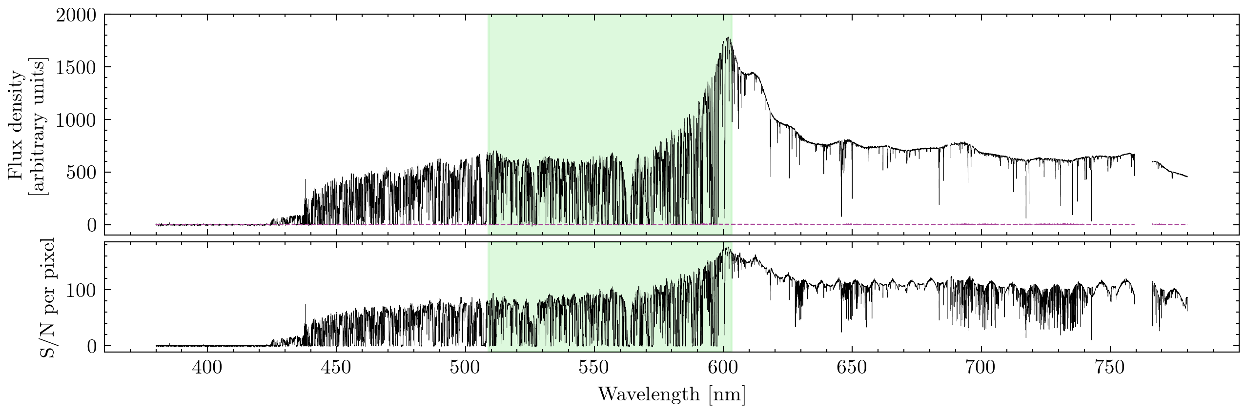 |
Quasar J0529-4351 high-energy observations: $L_{\rm bol} \sim 10^{48}$ erg/s accretion disk, SED decomposition, and Eddington limit | [[Astrostatistics]] |
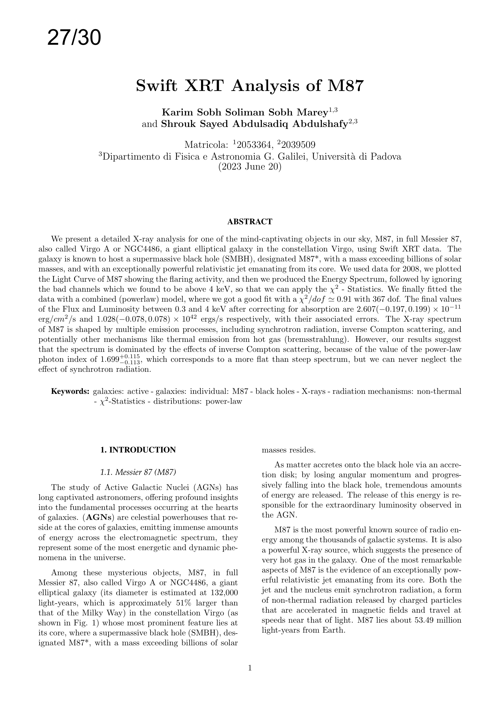 |
Swift XRT observation of M87: count map, PSF radial profile, light curve, or XSPEC powerlaw spectral fit | [[Point Spread Function (PSF)]] |
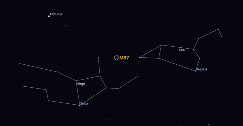 |
Swift XRT observation of M87: count map, PSF radial profile, light curve, or XSPEC powerlaw spectral fit | [[Point Spread Function (PSF)]] |
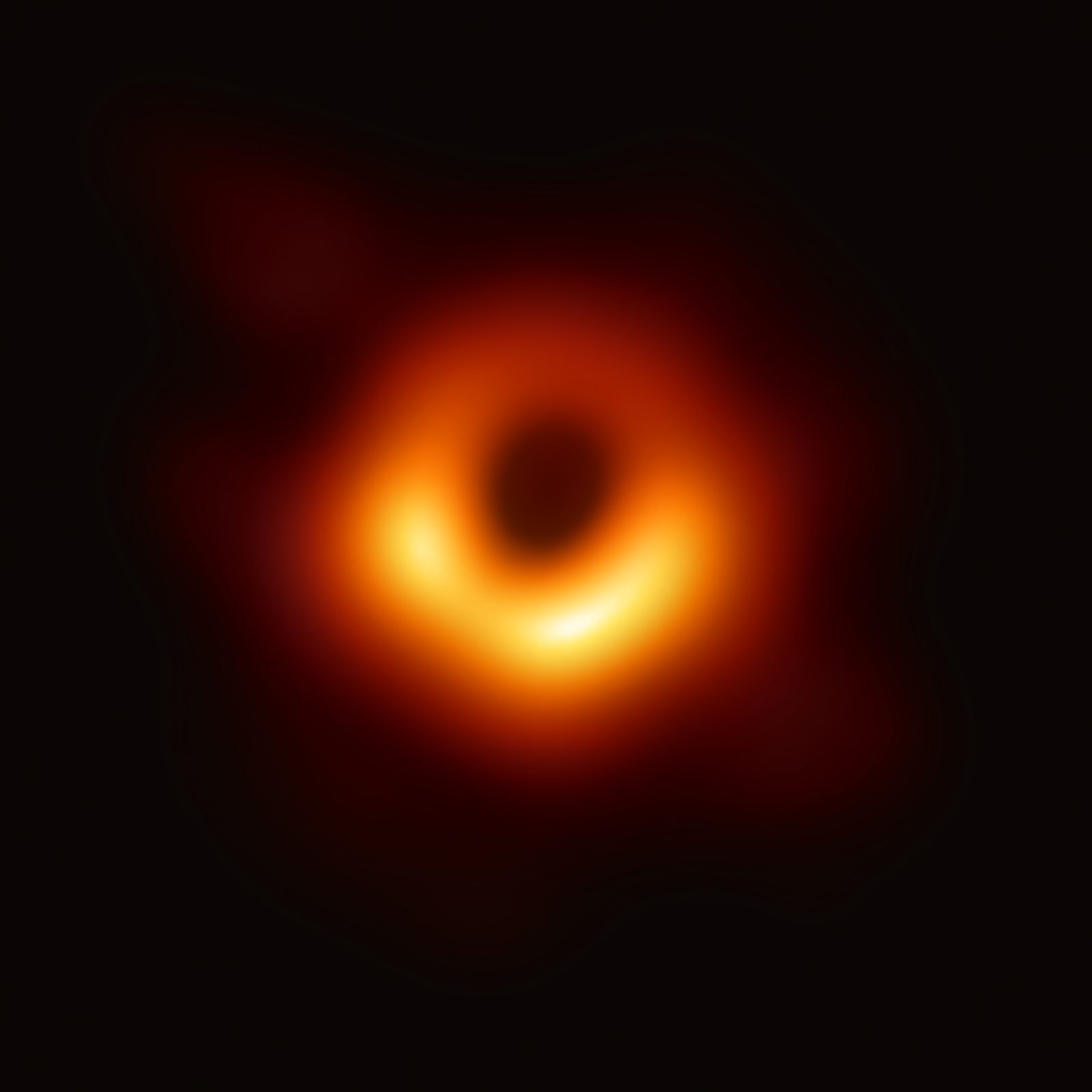 |
Swift XRT observation of M87: count map, PSF radial profile, light curve, or XSPEC powerlaw spectral fit | [[Point Spread Function (PSF)]] |
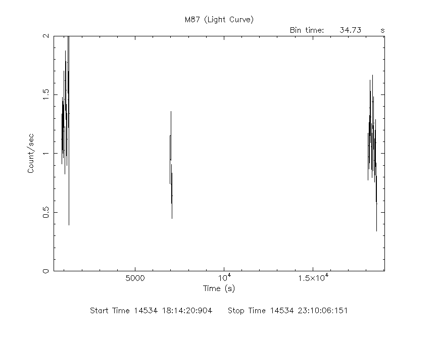 |
Swift XRT observation of M87: count map, PSF radial profile, light curve, or XSPEC powerlaw spectral fit | [[Point Spread Function (PSF)]] |
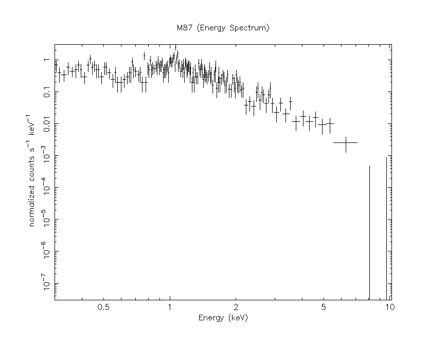 |
Swift XRT observation of M87: count map, PSF radial profile, light curve, or XSPEC powerlaw spectral fit | [[Point Spread Function (PSF)]] |
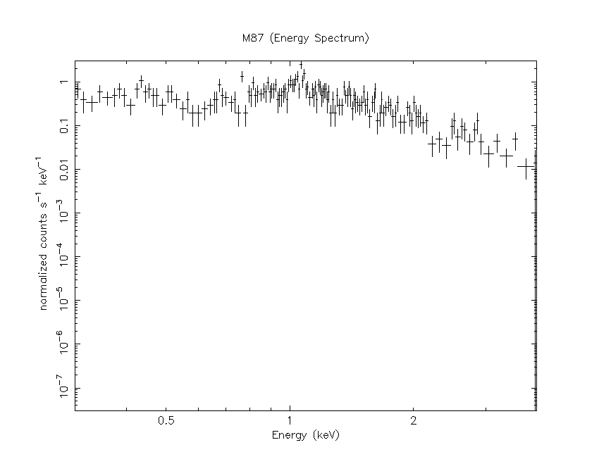 |
Swift XRT observation of M87: count map, PSF radial profile, light curve, or XSPEC powerlaw spectral fit | [[Point Spread Function (PSF)]] |
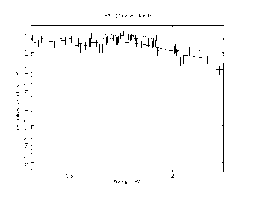 |
Swift XRT observation of M87: count map, PSF radial profile, light curve, or XSPEC powerlaw spectral fit | [[Point Spread Function (PSF)]] |
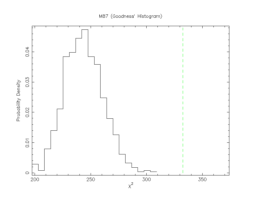 |
Swift XRT observation of M87: count map, PSF radial profile, light curve, or XSPEC powerlaw spectral fit | [[Point Spread Function (PSF)]] |
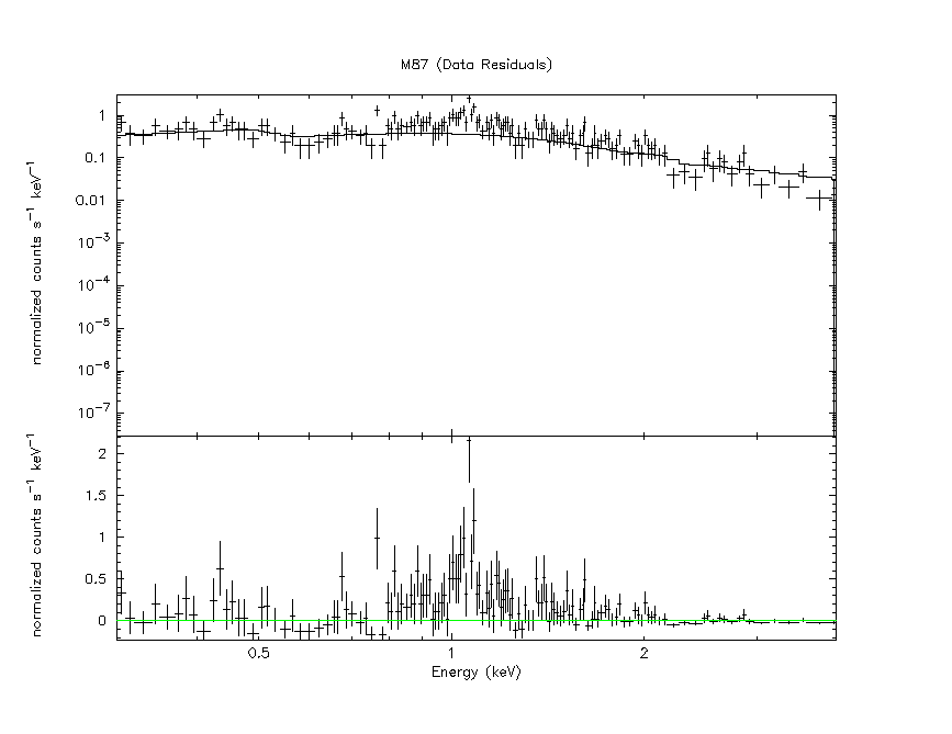 |
Swift XRT observation of M87: count map, PSF radial profile, light curve, or XSPEC powerlaw spectral fit | [[Point Spread Function (PSF)]] |
 |
XMM-Newton EPIC pn/MOS spectral fitting: ARF/RMF forward folding, Cash statistics, and Fe K$\alpha$ 6.4 keV line | [[Fitting]] |
 |
XMM-Newton EPIC pn/MOS spectral fitting: ARF/RMF forward folding, Cash statistics, and Fe K$\alpha$ 6.4 keV line | [[Fitting]] |
 |
XMM-Newton EPIC pn/MOS spectral fitting: ARF/RMF forward folding, Cash statistics, and Fe K$\alpha$ 6.4 keV line | [[Fitting]] |
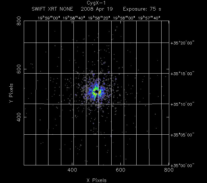 |
XMM-Newton EPIC pn/MOS spectral fitting: ARF/RMF forward folding, Cash statistics, and Fe K$\alpha$ 6.4 keV line | [[Fitting]] |
 |
X-ray CCD / Wolter Type-I optics: grazing reflection, split-event grades, pile-up, or quantum efficiency curve | [[CCDs for X-rays]] |
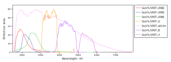 |
X-ray CCD / Wolter Type-I optics: grazing reflection, split-event grades, pile-up, or quantum efficiency curve | [[CCDs for X-rays]] |
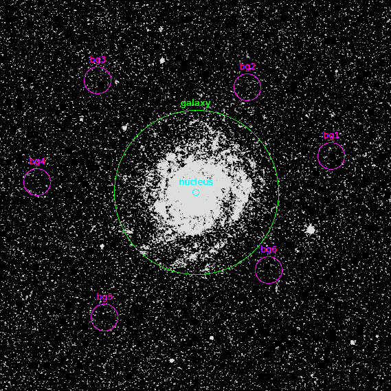 |
X-ray CCD / Wolter Type-I optics: grazing reflection, split-event grades, pile-up, or quantum efficiency curve | [[CCDs for X-rays]] |
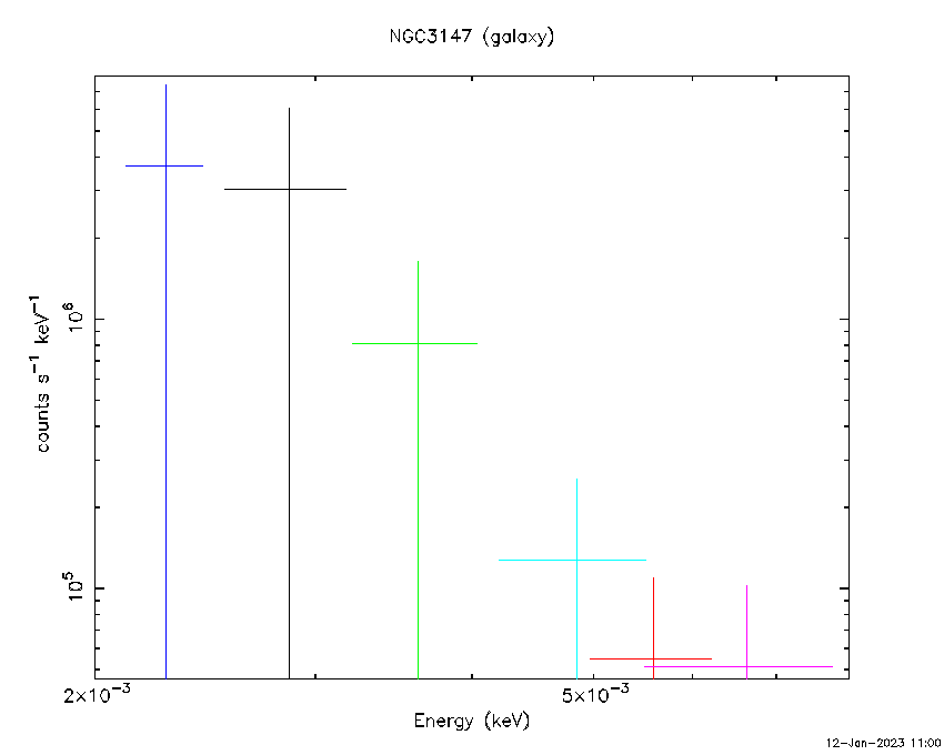 |
X-ray CCD / Wolter Type-I optics: grazing reflection, split-event grades, pile-up, or quantum efficiency curve | [[CCDs for X-rays]] |
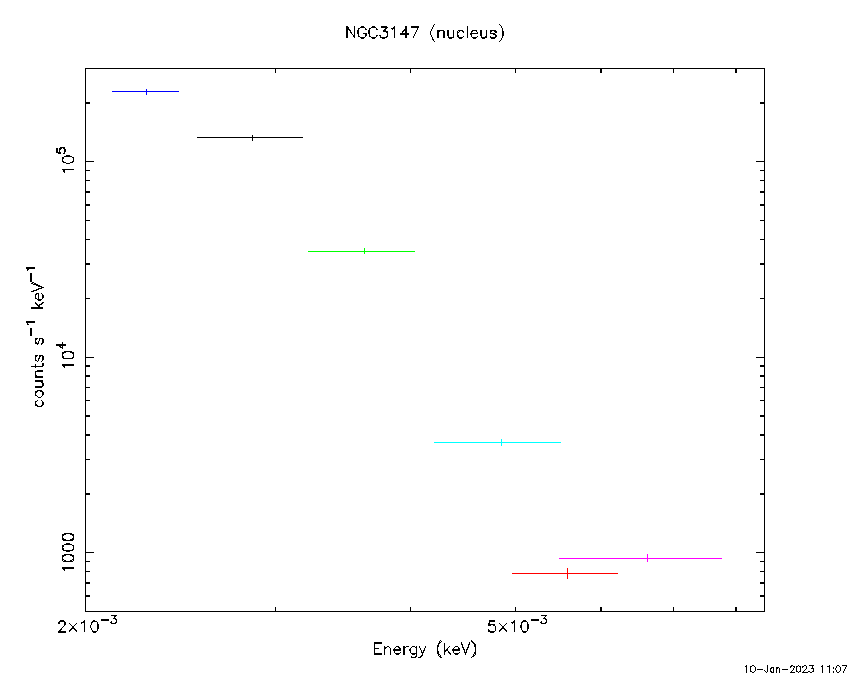 |
X-ray CCD / Wolter Type-I optics: grazing reflection, split-event grades, pile-up, or quantum efficiency curve | [[CCDs for X-rays]] |
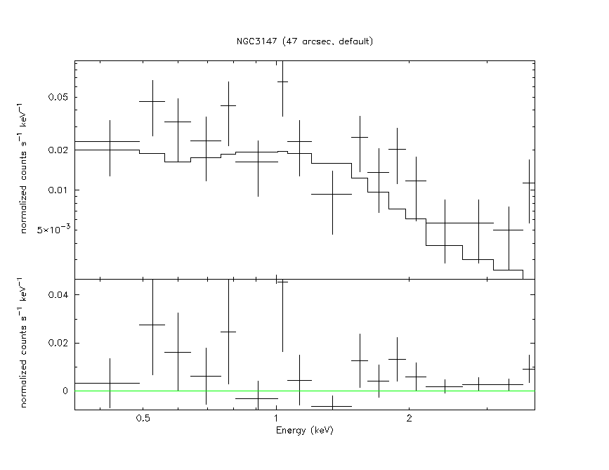 |
X-ray CCD / Wolter Type-I optics: grazing reflection, split-event grades, pile-up, or quantum efficiency curve | [[CCDs for X-rays]] |
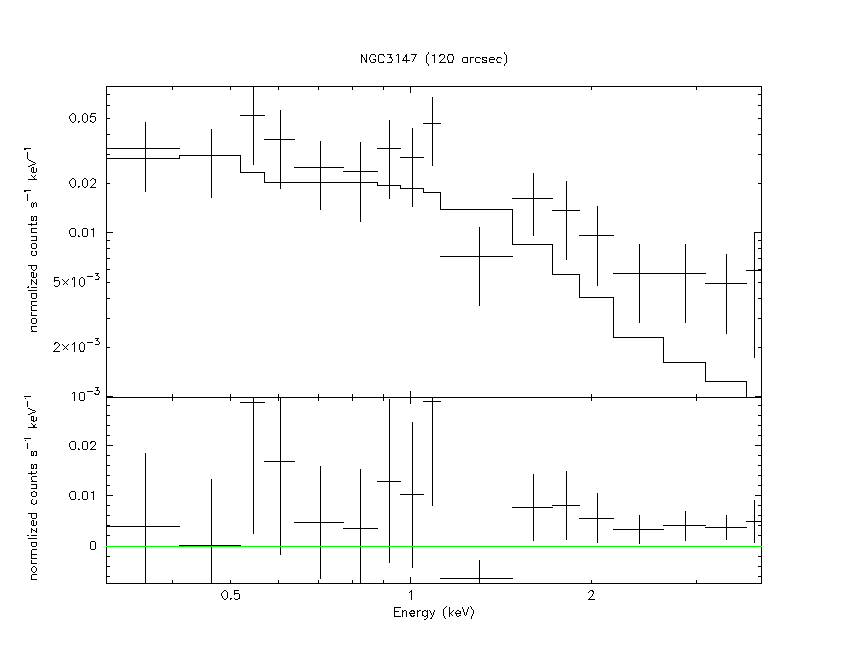 |
X-ray CCD / Wolter Type-I optics: grazing reflection, split-event grades, pile-up, or quantum efficiency curve | [[CCDs for X-rays]] |
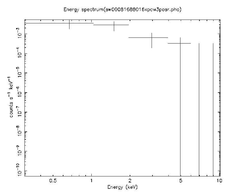 |
X-ray CCD / Wolter Type-I optics: grazing reflection, split-event grades, pile-up, or quantum efficiency curve | [[CCDs for X-rays]] |
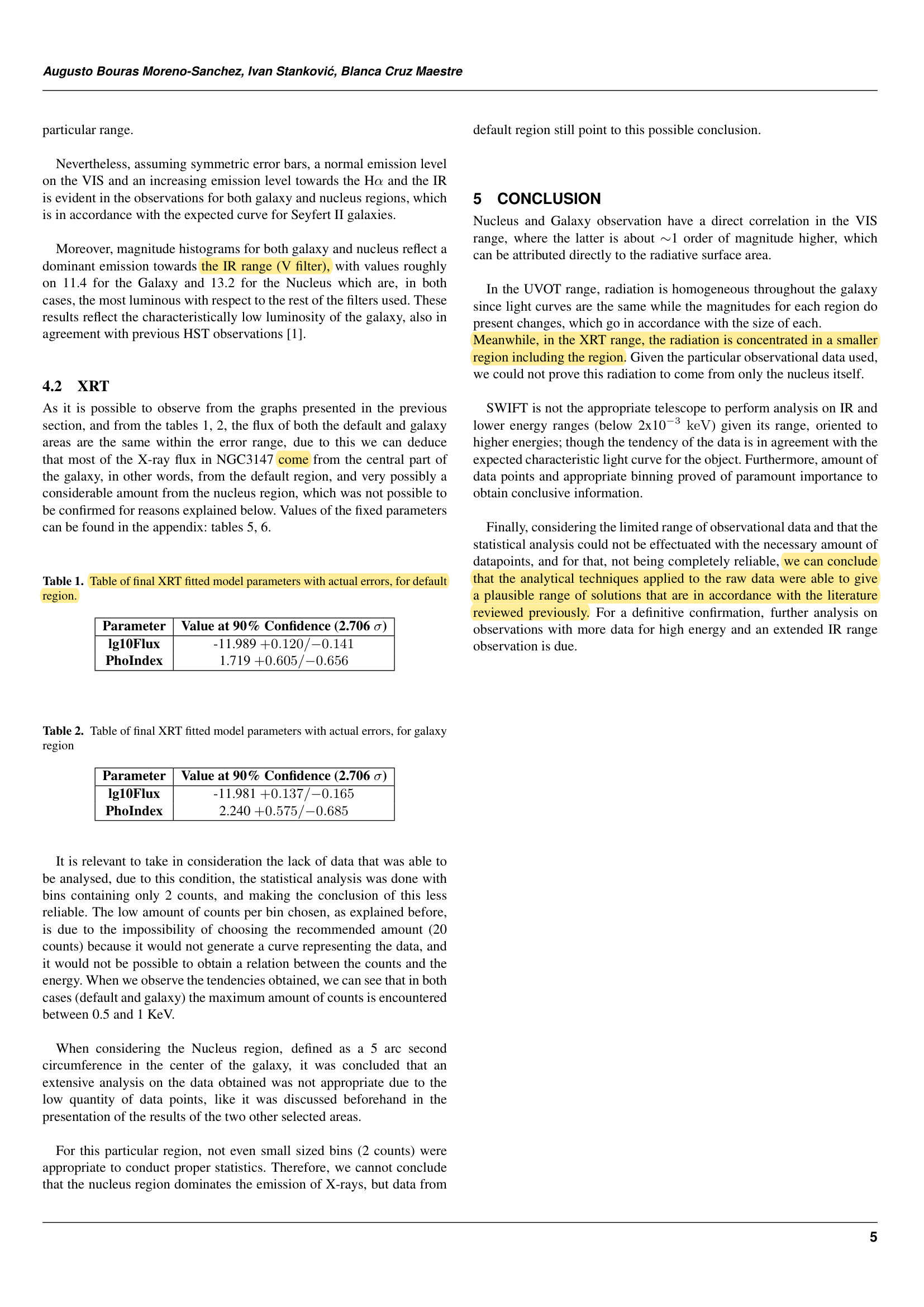 |
X-ray CCD / Wolter Type-I optics: grazing reflection, split-event grades, pile-up, or quantum efficiency curve | [[CCDs for X-rays]] |
Wikipedia and arXiv sources
Every zettel in this map ends with a short sourced section: a definition quoted from Wikipedia (44 zettels) or from the abstract of an arXiv review (5 zettels), and, where a free figure exists, the credited lead figure of the Wikipedia article (Wikimedia Commons) or a figure from an openly licensed arXiv paper. The lecture-slide figures above are unchanged.
| Zettel | Wikipedia | arXiv review | Figure |
|---|---|---|---|
| [[A Brief History of X-ray and Gamma-ray Missions]] | X-ray astronomy | Commons | |
| [[Accretion onto compact objects]] | Accretion (astrophysics) | Commons | |
| [[Angular Resolution]] | Angular resolution | Commons | |
| [[Appendix A - Optical telescopes]] | Optical telescope | ||
| [[Appendix B - Aberrations]] | Optical aberration | Commons | |
| [[Appendix C - Telescope configurations]] | Cassegrain reflector | Commons | |
| [[Appendix D - Gratings and spectrographs]] | Diffraction grating | Commons | |
| [[Appendix E - Astronomical coordinates]] | Astronomical coordinate systems | Commons | |
| [[Astrostatistics]] | Astrostatistics | ||
| [[Atmospheric transmission]] | Atmospheric window | Commons | |
| [[Blandford-Znajek Mechanism]] | Blandford–Znajek process | arXiv:1812.06025 | Commons |
| [[Bragg Reflection]] | Bragg’s law | ||
| [[Bremsstrahlung]] | Bremsstrahlung | Commons | |
| [[CCD readout]] | Charge-coupled device | Commons | |
| [[CCDs for X-rays]] | X-ray telescope | Commons | |
| [[Charge-Coupled Device]] | Charge-coupled device | Commons | |
| [[Coded Mask]] | Coded aperture | Commons | |
| [[Compton and Inverse Compton]] | Compton scattering | Commons | |
| [[Compton scattering and pair production]] | Pair production | Commons | |
| [[Compton Telescope]] | Compton telescope | Commons | |
| [[Distributions]] | Probability distribution | Commons | |
| [[Effective Area]] | Aperture (antenna) | ||
| [[Fitting]] | Curve fitting | Commons | |
| [[Grazing incidence]] | Wolter telescope | Commons | |
| [[Innermost Stable Circular Orbit ISCO]] | Innermost stable circular orbit | arXiv:gr-qc/9712019 | |
| [[Kerr Metric Horizon and Ergosphere Geometry]] | Kerr metric | arXiv:gr-qc/9712019 | Commons |
| [[Luminosity and Flux for -Instrumentations]] | Luminosity | Commons | |
| [[Luminosity]] | Luminosity | Commons | |
| [[Mechanical Collimator]] | Collimator | ||
| [[p-value]] | P-value | ||
| [[Photoelectric absorption]] | Photoelectric effect | Commons | |
| [[Point Spread Function (PSF)]] | Point spread function | Commons | |
| [[Processes of photon-matter interaction]] | Gamma ray | Commons | |
| [[Quantum efficiency]] | Quantum efficiency | Commons | |
| [[Radiative Processes]] | Radiative transfer | ||
| [[Rayleigh criterion]] | Angular resolution | Commons | |
| [[Relativistic Iron Line Profiles]] | Accretion disk | arXiv:1302.3260 | Commons |
| [[Seeing Effect]] | Astronomical seeing | arXiv:1201.5741 | Commons |
| [[Signal-Noise Ratio]] | Signal-to-noise ratio | Commons | |
| [[Synchroton]] | Synchrotron radiation | ||
| [[Telescope resolving power]] | Angular resolution | Commons | |
| [[The p-n junction]] | P–n junction | Commons | |
| [[Wolter Telescope]] | Wolter telescope | Commons | |
| [[X-ray diffraction grating]] | Diffraction grating | Commons |
High Energy Astrophysics Laboratory Oral Exam Defense Preparation Matrix
Question 1 - Grazing Incidence Reflection & The Wolter Type-I Telescope
- Blackboard Prompt: Why cannot conventional normal-incidence mirrors reflect X-rays? Derive the critical angle for total external reflection in the X-ray regime, and explain why two reflections (paraboloid + hyperboloid) are required in Wolter telescopes.
- Starting Equation: \(n = 1 - \delta + i\beta, \quad \delta = \frac{n_e r_e \lambda^2}{2\pi} = \frac{\rho N_A r_e \lambda^2}{2\pi}\frac{Z}{A}\)
- Derivation & Blackboard Walkthrough:
- In the X-ray regime ($E > 0.1$ keV), photon frequencies $\omega \gg \omega_{\rm plasma}$ exceed the binding energy of atomic electrons. Electrons respond as free damped oscillators with Drude refractive index $n < 1$. 2. Because $n < 1$, light traveling from vacuum ($n_1 = 1$) into the mirror material ($n_2 = 1 - \delta < 1$) encounters a medium of lower optical density.
- By Snell’s law: $\cos\alpha = n\cos\alpha’$, where $\alpha$ is the grazing angle measured from the mirror surface. Setting refracted angle $\alpha’ = 0$ gives the critical grazing angle: \(\cos\alpha_c = 1 - \delta \implies 1 - \frac{\alpha_c^2}{2} \approx 1 - \delta \implies \alpha_c = \sqrt{2\delta}\)
- In practical units: $\alpha_c \approx 10’ \frac{\sqrt{\rho\,[{\rm g/cm}^3]}}{E\,[{\rm keV}]}$. For gold/iridium ($\rho \sim 19-22$ g/cm$^3$), $\alpha_c \sim 1^\circ$ at 1 keV, and decreases inversely with photon energy $\alpha_c \propto 1/E$.
- A single paraboloid reflection focuses on-axis rays perfectly, but suffers severe off-axis coma aberration, violating the Abbe sine condition: $\frac{\sin\alpha_{\rm in}}{\sin\alpha_{\rm out}} \ne {\rm const}$.
- Hans Wolter (1952) proved that adding a second confocal hyperboloid reflection cancels primary coma, producing a wide, sharp field of view. Nested coaxial mirror shells maximize geometric collecting area $A_{\rm geo}$.
- Professor Trap Points:
- Trap: Measuring angles from the normal. In X-ray optics, $\alpha$ is ALWAYS measured from the surface plane (grazing angle), so total external reflection occurs when $\alpha < \alpha_c$!
Question 2 - X-ray CCD Physics, Energy Resolution, and Pile-Up
- Blackboard Prompt: How does an X-ray CCD measure the energy of an incoming photon directly without a dispersive grating? Derive the theoretical energy resolution and explain the physical origin and consequences of photon pile-up.
- Starting Equation: \(N_e = \frac{E_{\rm ph}}{w}, \quad w = 3.68\,{\rm eV} \text{ (silicon)}\)
- Derivation & Blackboard Walkthrough:
- In optical CCDs, each photon creates a single electron ($N_e = 1$). In X-rays, a photon (e.g. 1 keV) undergoes photoelectric absorption, producing a high-energy photoelectron that creates an ionization cascade of thousands of electron-hole pairs.
- In silicon, the average energy required to create an electron-hole pair is $w = 3.68$ eV (higher than bandgap 1.12 eV because energy is lost to phonons/lattice vibrations).
- The number of created electrons is proportional to photon energy: $N_e = E_{\rm ph}/w$. A 1 keV photon produces $N_e \approx 272$ electrons, a 6.4 keV Fe K$\alpha$ photon produces $N_e \approx 1739$ electrons.
- The statistical variance in $N_e$ is sub-Poissonian, quantified by the Fano factor $F \approx 0.115$ in silicon: $\sigma_{N_e}^2 = F \langle N_e \rangle = F \frac{E_{\rm ph}}{w}$.
- Total energy resolution FWHM accounting for readout noise $\sigma_{\rm RON}$: \(\Delta E_{\rm FWHM} = 2.355 w \sqrt{\sigma_{N_e}^2 + \sigma_{\rm RON}^2} = 2.355 \sqrt{F w E_{\rm ph} + (w\sigma_{\rm RON})^2}\) At 5.9 keV ($^{55}{\rm Fe}$ calibration source), $\Delta E_{\rm FWHM} \approx 120-130$ eV ($R = E/\Delta E \sim 45-50$).
- Photon Pile-Up: Occurs when two or more X-ray photons strike the same pixel (or neighboring pixels) within a single CCD readout frame time $\tau_{\rm frame}$ (e.g. 2.5 s in Swift PC mode).
- Consequences of pile-up:
- Grade migration: Multi-photon events are flagged as cosmic-ray tracks and discarded, causing flux loss.
- Spectral hardening: Two 1 keV photons are registered as a single 2 keV event, artificially shifting the fitted photon index $\Gamma$ to harder (lower) values.
- Diagnostics: A “hole” or depression in the central core of the PSF count map. Mitigation: Extract photons in an annular region excluding the piled-up core, or switch to Windowed Timing (WT) mode (1.7 ms frame time).
Question 3 - The Forward Folding Problem & Instrumental Calibration (ARF and RMF)
- Blackboard Prompt: Why is it mathematically impossible to directly invert an observed X-ray pulse-height spectrum to recover the sky spectrum? Explain the forward-folding process in XSPEC, defining the ARF and RMF matrices.
- Starting Equation: \(C(I) = t_{\rm exp} \int_0^\infty R(I, E) A(E) F(E) dE + B(I)\)
- Derivation & Blackboard Walkthrough:
- The detector registers discrete instrumental pulse-height channels $I$ (Pulse Invariant PI channels), not continuous physical energy $E$.
- Inverting $F(E) = [R A]^{-1} C(I)$ is an ill-conditioned, unstable Fredholm integral equation of the first kind. Small noise spikes in $C(I)$ produce catastrophic high-frequency oscillations in $F(E)$.
- Therefore, X-ray spectral analysis uses Forward Folding: propose a physical model $F(E; \vec{\theta})$ (e.g.
tbabs * powerlaw), fold it through the instrument response, and compare with observed counts $C(I)$. - Ancillary Response File (ARF), $A(E)$ [cm$^2$]: Contains the energy-dependent effective area: $A(E) = A_{\rm geo} \times R_{\rm mirror}^2(E) \times T_{\rm filter}(E) \times {\rm QE}(E) \times {\rm EEF}(r_{\rm src})$.
- Redistribution Matrix File (RMF), $R(I, E)$ [dimensionless]: The probability that a photon of true energy $E$ is detected in instrumental channel $I$. Encodes detector gain, energy resolution, escape peaks, and fluorescent sub-threshold losses.
- Fit Statistics: For high counts ($C_I \ge 20$), use Pearson $\chi^2$: $\chi^2 = \sum_I \frac{(C_I - M_I)^2}{\sigma_I^2}$. For low counts ($C_I < 20$), Poisson statistics govern, use the Cash statistic (C-stat): $C = 2 \sum_I (M_I - C_I \ln M_I)$, which avoids bias from artificial data binning.
Essential High Energy Laboratory Formulas Quick Sheet
| Quantity / Concept | Formula | Physical Meaning & Units |
|---|---|---|
| Critical Grazing Angle | $\alpha_c \approx \sqrt{2\delta} \approx 10’\frac{\sqrt{\rho}}{E_{\rm keV}}$ | Angle below which total external X-ray reflection occurs |
| Effective Collecting Area | $A_{\rm eff}(E) = A_{\rm geo} R^2(E) T_{\rm filter}(E) {\rm QE}(E)$ | Net effective collecting area at photon energy $E$ [cm$^2$] |
| CCD Electron Production | $N_e = \frac{E_{\rm ph}}{w}, \quad w = 3.68\,{\rm eV}$ | Mean number of electron-hole pairs produced in silicon |
| Fano Theoretical FWHM | $\Delta E_{\rm FWHM} = 2.355\sqrt{F w E_{\rm ph} + (w\sigma_{\rm RON})^2}$ | Energy resolution of silicon detector, Fano factor $F \approx 0.115$ |
| Forward Folding Integral | $C(I) = t \int R(I, E) A(E) F(E) dE$ | Expected channel count rate from true sky flux $F(E)$ |
| Cash Statistic (C-stat) | $C = 2 \sum_{i=1}^N (M_i - C_i \ln M_i)$ | Maximum likelihood parameter estimator for Poisson counts |
| Photoelectric Cross-Section | $\sigma_{\rm ph}(E) \propto Z^4 E^{-3}$ | Dominant soft X-ray absorption mechanism in cool ISM |
| Absorption Transmission | $T(E) = e^{-N_H \sigma_{\rm ISM}(E)}$ | ISM continuum attenuation factor, $N_H$ = neutral H column density |
| Power-Law Photon Flux | $F(E) = K E^{-\Gamma}$ | Continuum emission model, $\Gamma = \alpha + 1$ (photon index) |
| Eddington Luminosity | $L_{\rm Edd} = \frac{4\pi G M m_p c}{\sigma_T} \approx 1.26 \times 10^{38}\left(\frac{M}{M_\odot}\right)\,{\rm erg/s}$ | Maximum radiation-balanced steady accretion luminosity |
Follow along on Instagram @your.astrophysicist · Report an issue