General_Relativity_MOC
General Relativity for Astrophysics and Cosmology, Map of Content
A.Y. 2025/2026, Prof. Francesco D’Eramo (SCQ0093378), University of Padua. Master’s-level course taught in the first semester. The exam (oral, with written portion) draws from a published list of 20 questions.
the question this whole course is trying to answer
before any equations, before any tensors, before any of the machinery, here is the question I want to keep in my head for the entire course:
what is gravity, really?
Newton answered: gravity is a force, like electricity. masses pull on each other across empty space, instantly, with strength $GMm/r^2$. this works cleanly for almost everything: cannonballs, planets, satellites, the moon. it is the most successful theory in the history of physics until 1916.
but Newton’s answer has two cracks in it.
crack one, the Mercury problem. Mercury’s orbit precesses (the ellipse rotates slightly each year), and Newton predicts $532$ arcseconds per century from the pull of the other planets. observations give $575$. there is an extra $43’’/$century that no one can explain. Le Verrier (the same astronomer who predicted Neptune from Uranus’s wobble) tried to fit it with a hypothetical inner planet, “Vulcan.” Vulcan does not exist. Mercury’s extra precession just sits there, an embarrassment, for fifty years.
crack two, the speed-of-light problem. Einstein’s special relativity (1905) says nothing travels faster than $c$. but Newton’s gravity propagates instantly, the moment the sun moved, Earth would feel it immediately, with no delay. either Einstein is wrong or Newton is wrong. they cannot both be right.
Einstein spent ten years (1905 to 1915) figuring out a new theory of gravity that fixes both problems. that theory is general relativity, GR, the subject of this course. its answer to “what is gravity, really?” is one of the nicest ideas in physics:
gravity is not a force. gravity is what spacetime looks like when there is matter in it. objects in free fall just follow the natural straight lines of the curved spacetime around them. and the curving of spacetime is what we have always called “the pull of gravity.”
that is the whole course in one sentence. everything else is the math we need to make this concrete.
the chain of objects, what we will build
GR’s mathematical machinery is one chain. start with a metric (the geometry of spacetime), differentiate it carefully to get curvature, contract it to get something matter can source, and equate it to matter. the chain looks like this:
\[g_{\mu\nu} \;\longrightarrow\; \Gamma^{\alpha}{}_{\mu\nu} \;\longrightarrow\; R^{\alpha}{}_{\beta\mu\nu} \;\longrightarrow\; R_{\mu\nu} \;\longrightarrow\; R \;\longrightarrow\; G_{\mu\nu} = 8\pi G\, T_{\mu\nu}\]let me say what each of these things is, in plain English, in the order I will meet them.
$g_{\mu\nu}$ the metric, is the rulebook for measuring distances and times in spacetime. in flat space it is just Pythagoras: $ds^2 = dx^2 + dy^2 + dz^2$. in curved spacetime it is more complicated. it is what i write down when i describe a spacetime: Schwarzschild has one, FLRW has one, Kerr has one. the metric is the spacetime, in the same way that a function on the real line is the same as its graph.
$\Gamma^\alpha{}_{\mu\nu}$ the Christoffel symbols, tell me how my coordinate axes tilt as i move around. in flat space using cartesian coordinates they are zero, the axes never tilt. in flat space using polar coordinates they are non-zero, the radial and angular directions twist around as i go around the origin. on a curved manifold they are non-zero too, but for a different reason: the manifold itself is curving the axes. Christoffels are the price i pay for using coordinates.
$R^\alpha{}_{\beta\mu\nu}$ the Riemann tensor, is the actual curvature of the spacetime. it asks: if i carry a vector around a tiny closed loop, does it come back to the same vector? in flat space, yes. in curved space, no, it comes back rotated. Riemann measures how much. it is the “shape” of curvature.
$R_{\mu\nu}$ the Ricci tensor and $R$ the Ricci scalar, are simpler summaries of Riemann. you take certain “averages” (contractions) over Riemann’s many indices. Ricci has fewer pieces of information, but those pieces are the ones matter cares about.
$G_{\mu\nu}$ the Einstein tensor, is built from Ricci and the metric in a very specific way that makes it conserved. if i set it equal to the matter content $T_{\mu\nu}$ (energy density, pressure, momentum), i get the field equations of GR:
\[G_{\mu\nu} = 8\pi G\, T_{\mu\nu}\]this single equation is what runs the universe.
so the whole course is: what is $g$, how do i get $\Gamma$ from $g$, how do i get $R$ from $\Gamma$, how does Einstein’s equation connect $R$ to matter, and what physics falls out when i solve it.
the two halves of GR, told as a sentence
a famous summary by John Wheeler:
matter tells spacetime how to curve, spacetime tells matter how to move.
these are the two halves of the theory and they are decoupled in a way:
- matter tells spacetime how to curve is Einstein’s equation, $G_{\mu\nu} = 8\pi G T_{\mu\nu}$. it is one equation (well, ten) saying: given a distribution of matter and energy, here is what the geometry has to be.
- spacetime tells matter how to move is the geodesic equation, $\ddot x^\mu + \Gamma^\mu{}_{\alpha\beta}\dot x^\alpha \dot x^\beta = 0$. it says: in a given geometry, freely-falling particles follow these specific paths.
the two halves connect through the metric. matter sources curvature in the metric (Einstein), then the curved metric determines how matter moves (geodesic). the loop closes through the metric.
how to use this map
this MOC is the spine of my GR study. every blue link drops into a single concept note that I can read in a sitting. the structure i recommend:
- read this entire MOC top to bottom to get the big picture
- for each block, read the linked Baumann chapter note to get the conceptual story (
02_Literature/Book/Baumann GR/) - for each exam question, read the question walkthrough in
05_Projects/Exam/First Year/GR Exam 2026/ - at the end of each block, write down the chain by hand: metric, Christoffels, Riemann, what the question asks, what the answer is
every concept note follows the same teaching order: motivation, analogy, definition, what it means, example, why it matters for the exam.
block 0, before we start
these are not equations, they are the rules and the conventions.
- GR exam rules what the exam looks like, the 20-question system, what is allowed
- GR equation sheet the official formula sheet, organized for fast lookup
- [[Baumann GR]] reading companion to the textbook, chapter by chapter
block 1, the language, what spacetime is and how to write it
before we can do anything, we have to agree on a language for “spacetime as a geometric object.” this is differential geometry. it sounds intimidating but the idea is simple: a curved space (like the surface of the Earth) can be described locally by patches of coordinates that we sew together. we put a metric on top to measure distances. we define vectors and tensors that live on the space without depending on which coordinates we picked.
physical question this block answers: how do i write down a spacetime so that i can do calculus on it?
- [[Manifold metric and signature]] what is a manifold, what is a metric, why “Lorentzian signature” matters
- [[Coordinate transformations and tensors]] vectors, co-vectors, tensors, why partial derivatives are not tensors
- [[Locally inertial frame]] the GR version of “Newton’s first law works locally”
- [[Christoffel symbols]] the price of using coordinates in curved space
- [[Levi-Civita connection]] why GR uses one specific connection and not others
- [[Covariant derivative]] the differentiation that respects curvature
- [[Metric compatibility]] why $\nabla g = 0$ and why this matters
- [[Parallel transport]] the curved-space version of “translating without rotating”
questions in this block: Q1 - Christoffels for diagonal 2D metric, Q2 - Christoffels for radial 2D metric, Q3 - covariant derivatives in polar, Q4 - metric compatibility on the 2-sphere.
reading: [[Ch 1 - Gravity is Geometry]] for the motivation, [[Ch 2 - Some Differential Geometry]] for the math.
block 2, curvature, what it actually means for space to be “curved”
now that we have the language, what is “curvature”? the question matters because Newton’s gravity has nothing like it: in Newton, space is flat and gravity is a force on top of flatness. in GR, space itself bends. what does that mean operationally?
physical question this block answers: how do i know if a space is curved, and how do i quantify it?
the answer is the Riemann tensor. it is built from an operational test: parallel transport a vector around a tiny closed loop. if the vector comes back to the same vector, the space is flat. if it comes back rotated, the space is curved, and Riemann measures how much. this is not a metaphor. it is the actual definition.
- [[Riemann tensor]] the path-dependence of parallel transport, made precise
- [[Riemann tensor symmetries]] the four symmetries (antisym pair, antisym pair, pair exchange, first Bianchi) that reduce its components
- [[Counting Riemann components]] $n^2(n^2-1)/12$, equals 1 in 2D, 6 in 3D, 20 in 4D
- [[Ricci tensor and scalar]] the contractions, what they capture
- [[Sectional and Gaussian curvature]] the geometric meaning of one Riemann component
- [[Bianchi identities]] the differential identity that forces conservation laws
- [[Geodesic deviation]] the physical content of curvature: tidal forces
questions in this block: Q5 - Riemann for 1+1 expanding metric, Q6 - Riemann for conformally flat 1+1.
reading: [[Ch 4 - Spacetime Curvature]].
block 3, geodesics, how matter moves through curved spacetime
a geodesic is the curved-space version of a “straight line.” in flat space, an unaccelerated particle moves in a straight line, the shortest path between two points. in curved space, an unaccelerated (free-falling) particle moves in a geodesic, which is still the “straightest” possible path locally but globally can curve back on itself.
physical question this block answers: given a spacetime, what paths do free particles take?
three equivalent ways to think about a geodesic:
- it is the path that extremizes proper time (or proper length)
- it is the path that parallel-transports its own tangent vector
- it is the path that satisfies the geodesic equation $\ddot x + \Gamma \dot x \dot x = 0$
definition 1 connects to Lagrangian mechanics ($S = -m \int d\tau$). definition 2 connects to the parallel-transport machinery from Block 2. definition 3 is the explicit ODE i actually solve.
a deep simplification: when the spacetime has symmetries (the metric does not depend on some coordinate), there are conserved quantities along the geodesic. this is the GR version of Noether’s theorem and it lets me reduce 4D problems to 1D effective-potential problems.
- [[Geodesic equation]] the ODE for free-falling motion
- [[Affine parameter]] proper time for massive, anything-linear for null
- [[Killing vectors and conserved quantities]] when the metric has a symmetry, there is a conserved momentum
- [[Effective potential approach]] reducing the 4D Schwarzschild geodesic to a 1D radial problem
- [[Timelike vs null vs spacelike]] the three flavors of geodesic
questions in this block: Q7 - geodesics on the 2-sphere, Q8 - null geodesic in static metric.
reading: [[Ch 3 - A First Look at Geodesics]] (gives a great pedagogical derivation of the geodesic equation from the relativistic action).
block 4, Einstein’s equation, how matter sources curvature
we now have the language (Block 1), the curvature object (Block 2), and the equation of motion (Block 3). what we still need is the field equation: the analog of Maxwell’s equations for gravity. Einstein looked for it for nearly ten years.
physical question this block answers: given a distribution of matter and energy, what is the spacetime?
the answer comes out by trial. Einstein’s first guess was $R_{\mu\nu} = 8\pi G T_{\mu\nu}$ (Ricci tensor sources stress-energy). this fails because Ricci is not automatically conserved while stress-energy is. fixing it requires the Einstein tensor
\[G_{\mu\nu} \equiv R_{\mu\nu} - \tfrac12 g_{\mu\nu} R\]which by the contracted Bianchi identity satisfies $\nabla^\mu G_{\mu\nu} = 0$ identically. Einstein’s equation is then
\[G_{\mu\nu} = 8\pi G T_{\mu\nu}\]the constant $8\pi G$ is fixed by demanding the equation reduces to Newton in the appropriate limit.
- [[Einstein equations]] the master equation
- [[Einstein tensor and Bianchi]] why it has to be $G$ and not $R$
- [[Stress-energy tensor]] perfect fluid, dust, radiation, vacuum, scalar field
- [[Trace-reversed Einstein equations]] the equivalent form $R_{\mu\nu} = 8\pi G(T_{\mu\nu} - \tfrac12 g_{\mu\nu}T)$
- [[Cosmological constant]] the only other thing that can be added consistently
reading: [[Ch 5 - The Einstein Equation]].
block 5, Schwarzschild, the gravitational field of a star or black hole
with Einstein’s equation in hand, we can finally solve for some real spacetimes. the simplest non-trivial case is the gravitational field outside a spherically symmetric, non-rotating mass: a star, a planet, a non-rotating black hole. the solution is the Schwarzschild metric, and it is one of the most important objects in physics.
physical question this block answers: what is the spacetime around a spherical mass, and what does this predict about orbits and light?
four physical predictions, all confirmed by experiment:
- orbits precess (Mercury, $43’’$/century)
- light bends (Sun, $1.75’’$, Eddington 1919)
- there is an innermost stable circular orbit (ISCO at $r = 6GM$, sets the inner edge of accretion disks)
- there is a photon sphere (unstable circular photon orbit at $r = 3GM$, the bright ring in EHT images of black holes)
a fifth prediction: there is an event horizon at $r = 2GM$, a one-way membrane. inside it, even light cannot escape. that is the black hole.
- [[Schwarzschild metric]] the metric and its derivation
- [[Birkhoff theorem]] spherically symmetric vacuum is automatically static
- [[Schwarzschild Christoffels]] the standard table
- [[Schwarzschild horizon]] the $r = 2GM$ surface, why it is a coordinate singularity not a curvature one
- [[Schwarzschild effective potential]] the master tool for orbits
- [[Circular orbits in Schwarzschild]] $\Omega^2 = GM/r^3$ exactly
- [[Photon sphere]] $r = 3GM$, the bright ring
- [[Radial infall]] the cycloid solution
- [[Photon trajectories and impact parameter]] $b = L/E$ and $b_{\rm crit} = 3\sqrt{3}\,GM$
- [[Perihelion precession]] the $43’’$/century
- [[Light deflection]] the $1.75’’$
- [[Eddington-Finkelstein and Kruskal]] coordinates that pass through the horizon smoothly
beyond this course’s syllabus (not examined here, but the natural rotating generalization, used heavily in [[Lab_High-Energy_MOC]]): [[Kerr Metric Horizon and Ergosphere Geometry]] and [[Innermost Stable Circular Orbit ISCO]] generalize the $r=6GM$ Schwarzschild ISCO above to a spin-dependent $r_{\rm ISCO}(a_*)$ ranging from $M$ to $9M$.
questions in this block: Q11 - selected Schwarzschild Christoffels, Q12 - circular orbits and orbital frequency, Q13 - radial infall and proper time, Q14 - photon trajectory and impact parameter.
reading: [[Ch 5 - The Einstein Equation]] (Schwarzschild derivation), [[Ch 6 - Black Holes]] (deep cuts on horizons, Kruskal, Penrose diagrams).
block 6, linearized gravity, GR for weak fields
GR is a non-linear theory. the equations are notoriously hard to solve. but in many real situations the field is weak, the spacetime is “almost flat” with a small perturbation. then we can linearize and the equations become tractable.
physical question this block answers: how do i do GR perturbation theory?
write the metric as $g_{\mu\nu} = \eta_{\mu\nu} + h_{\mu\nu}$ with $\lvert h\rvert \ll 1$, keep only first-order terms in $h$. this regime contains:
- Newtonian gravity: the slow-motion, weak-field limit recovers Newton with $h_{00} = -2\Phi$
- gravitational waves: vacuum solutions of linearized GR
linearized GR has a gauge symmetry, just like electromagnetism. an infinitesimal coordinate change shifts $h_{\mu\nu}$ by $h \to h + 2\partial_{(\mu}\xi_{\nu)}$. fixing this gauge (Lorenz gauge, then transverse-traceless) is what makes the wave equation clean.
- [[Linearized metric perturbation]] $h_{\mu\nu}$ on Minkowski
- [[Linearized Christoffel and Riemann]] drop $\Gamma\Gamma$ terms
- [[Linearized gauge transformations]] residual diffeomorphism freedom
- [[Trace-reversed perturbation]] $\bar h_{\mu\nu} = h_{\mu\nu} - \tfrac12 \eta_{\mu\nu} h$, an involution
- [[Lorenz gauge]] $\partial^\mu \bar h_{\mu\nu} = 0$, makes Einstein’s equation a wave equation
- [[Newtonian limit of GR]] $h_{00} = -2\Phi$ recovers Poisson’s equation
- [[SVT decomposition]] scalar / vector / tensor split
questions in this block: Q9 - weak-field Christoffel Gamma_i_00, Q10 - weak-field Ricci scalar, Q15 - trace-reversed perturbation and Lorenz gauge.
reading: [[Ch 8 - Gravitational Waves]] § 8.1 for the linearized formalism.
block 7, gravitational waves, ripples in spacetime
vacuum solutions of linearized GR. the equations $\Box \bar h_{\mu\nu} = 0$ admit traveling wave solutions, gravitational waves. they propagate at the speed of light, carry energy, and were directly detected by LIGO in 2015.
physical question this block answers: what are gravitational waves and what do they do?
after fixing all the gauge freedom (Lorenz first, then four extra TT conditions), only two physical polarizations survive: $h_+$ (“plus”) and $h_\times$ (“cross”). they affect a ring of test masses by alternately stretching and squeezing it: the “+” pattern stretches the ring along $x$ while squeezing along $y$, then reverses. the “×” pattern is the same rotated by $45°$. LIGO detects this stretching directly through laser interferometry.
- [[Transverse traceless gauge]] the canonical GW gauge, four extra conditions, two polarizations
- [[Plus and cross polarizations]] $h_+, h_\times$, the stretching and squeezing patterns
- [[Geodesic deviation under a GW]] the LIGO physics, $\Delta L/L \sim h$
- [[Quadrupole formula]] $h^{TT}{ij} = (2G/r) \ddot Q{ij}$, why no monopole or dipole GW
- [[GW energy and angular momentum]] the Isaacson tensor
questions in this block: Q16 - Christoffels for a TT plane wave, Q17 - Riemann R_0x0x for a TT plane wave.
reading: [[Ch 8 - Gravitational Waves]] § 8.2 to 8.4.
block 8, FLRW cosmology, the universe as a dynamical system
the cosmological principle says the universe is homogeneous (same at every point) and isotropic (same in every direction) on large scales. plugging this assumption into Einstein’s equations gives the FLRW metric and the Friedmann equations. the result: the universe is one giant geodesic problem with one scale factor $a(t)$.
physical question this block answers: how does the universe evolve?
Friedmann equations:
\[H^2 = \frac{8\pi G}{3}\rho - \frac{k}{a^2}, \qquad \frac{\ddot a}{a} = -\frac{4\pi G}{3}(\rho + 3p)\]stress-energy conservation gives the continuity equation $\dot \rho + 3H(\rho + p) = 0$. with an equation of state $p = w\rho$, fluids dilute as $\rho \propto a^{-3(1+w)}$. matter ($w = 0$) dilutes as $a^{-3}$ (volume), radiation ($w = 1/3$) as $a^{-4}$ (volume + redshift), dark energy ($w = -1$) stays constant.
three eras of cosmic history:
- radiation era, $a \propto t^{1/2}$, until $z_{\rm eq} \sim 3400$
- matter era, $a \propto t^{2/3}$, until $z \sim 0.5$
- dark energy era, $a \propto e^{H_\Lambda t}$, now and forever
today: $\Omega_r \approx 9 \times 10^{-5}$, $\Omega_m \approx 0.32$, $\Omega_\Lambda \approx 0.68$, $\lvert\Omega_k\rvert < 0.005$. 5% baryons, 27% dark matter, 68% dark energy. 95% of the universe is invisible.
- [[Cosmological principle]] homogeneous + isotropic at each time
- [[FLRW metric]] $ds^2 = -dt^2 + a(t)^2 \gamma_{ij} dx^i dx^j$
- [[Spatial curvature parameter k]] flat / closed / open
- [[Friedmann equations]] the master cosmological equations
- [[Continuity equation]] from $\nabla^\mu T_{\mu\nu} = 0$
- [[Equation of state and density scaling]] $\rho \propto a^{-3(1+w)}$
- [[Cosmic eras]] radiation, matter, dark energy
- [[Matter radiation equality]] $a_{\rm eq}$, the cosmic transition
- [[Deceleration parameter]] $q$, why it is negative today
questions in this block: Q18 - derive the acceleration equation, Q19 - radiation universe, Q20 - matter plus radiation universe.
reading: [[Ch 7 - Cosmology]].
the 20 exam questions, with the topic each one tests
every question is a calculation that lives inside one of the eight blocks. when i prepare each one, i should think: which block? which physical concept? then the calculation falls out.
foundations (Christoffel, covariant derivative, metric compatibility):
- Q1 - Christoffels for diagonal 2D metric practice with the formula
- Q2 - Christoffels for radial 2D metric the universal 2D radial result
- Q3 - covariant derivatives in polar computing $\nabla V$ in flat-space polar
- Q4 - metric compatibility on the 2-sphere verifying $\nabla g = 0$ component by component
curvature:
- Q5 - Riemann for 1+1 expanding metric mini-FLRW Riemann
- Q6 - Riemann for conformally flat 1+1 the metric is secretly flat
geodesics:
- Q7 - geodesics on the 2-sphere meridians and the equator
- Q8 - null geodesic in static metric using $E$ and the null condition
linearized gravity:
- Q9 - weak-field Christoffel Gamma_i_00 reproduce Newton from GR
- Q10 - weak-field Ricci scalar $R = 2\nabla^2 \Phi$, recover Poisson
Schwarzschild:
- Q11 - selected Schwarzschild Christoffels the standard table
- Q12 - circular orbits and orbital frequency Kepler from Schwarzschild
- Q13 - radial infall and proper time cycloid solution
- Q14 - photon trajectory and impact parameter orbit equation $(dr/d\phi)^2$
gauge and waves:
- Q15 - trace-reversed perturbation and Lorenz gauge gauge transformation, reachability
- Q16 - Christoffels for a TT plane wave $\Gamma^x{}{0x}$, $\Gamma^x{}{zx}$
- Q17 - Riemann R_0x0x for a TT plane wave tidal force of the wave
cosmology:
- Q18 - derive the acceleration equation from Friedmann + continuity
- Q19 - radiation universe $\rho(a)$, $a(t)$, $H(t)$
- Q20 - matter plus radiation universe $\rho_m(a)$, $\rho_r(a)$, $a_{\rm eq}$
Literature & Primary Sources
Canonical and modern arXiv gr-qc/astro-ph.HE benchmark papers underlying the Kerr-metric and gravitational-wave physics above.
- [[Bardeen_Press_Teukolsky_1972_Rotating_Black_Holes|Bardeen, Press & Teukolsky (1972) - Rotating Black Holes]] - locally nonrotating frames, the ISCO formula, accretion efficiency
- [[Abbott_2016_LIGO_GW150914_Detection|Abbott et al. / LIGO & Virgo (2016) - Observation of Gravitational Waves (GW150914)]] - chirp-mass inspiral, merger, ringdown
- [[EHT_Collaboration_2022_Testing_Kerr_Metric_SgrA|Event Horizon Telescope Collaboration (2022) - Testing the Black Hole Metric (Sgr A*)]] - shadow-size Kerr test across mass scales
connections to other courses
GR is the geometric trunk that other courses graft onto.
- [[Observational_Cosmology_MOC]] is the same Block 8 (FLRW + Friedmann), but turned outward toward observation. distance ladders, the K-correction, surface-brightness dimming, the CMB, all sit on top of FLRW. when i derive Friedmann here, i am building the foundation that course needs.
- [[Lab_High-Energy_MOC]] turns Schwarzschild into observables. ISCO sets the inner edge of accretion disks (and hence the $L_{\rm Edd}$-scale luminosity). the photon sphere becomes the bright ring in EHT images. gravitational redshift shows up in iron K$\alpha$ line shapes from neutron stars and BHs.
- Fundamentals of Astrophysics and Cosmology (the parallel course): Newtonian-fluid derivation of Friedmann, and the basics of CMB physics. it is GR cosmology’s “easier sister.” i should read both side by side.
personal study notes
- GR by Jessica notes my own running notes
- Lez 4 13102025 · Lez 5 14012025 4Velocity · Lez 7 21102025 Energy momentum · Lez 10 3112025 Curvilinear lecture notes from class
sources and references
- Sean Carroll, Spacetime and Geometry the standard rigorous treatment, source for most of the equation sheet
- Bernard Schutz, A First Course in General Relativity more physical, intuition-first
- Daniel Baumann, General Relativity the book the course follows. reading companion (chapter by chapter) at [[Baumann GR]]
- 20 official questions:
Downloads/GR_Exam_2026.pdf - official equation sheet:
Downloads/GR_Equations_2026.pdf - long-form course walkthrough:
1st Semester/GENERAL RELATIVITY FOR ASTROPHYSICS AND COSMOLOGY/QA GR.pdf
the one-paragraph version of the entire course, for emergency oral situations
general relativity replaces Newton’s “gravity is a force” with “gravity is geometry.” spacetime is a Lorentzian manifold whose metric $g_{\mu\nu}$ encodes how distances are measured. coordinate axes generally tilt as i move around, captured by the Christoffel symbols $\Gamma^\alpha{}{\mu\nu}$, the unique symbols that are both metric-compatible and torsion-free. true curvature is captured by the Riemann tensor, defined by the path-dependence of parallel transport, and physically by the relative acceleration of nearby geodesics (tidal forces). matter sources curvature through Einstein’s equation $G{\mu\nu} = 8\pi G T_{\mu\nu}$, where $G_{\mu\nu} = R_{\mu\nu} - \tfrac12 g_{\mu\nu}R$ is the unique “second-derivative of metric” combination that is automatically conserved. matter responds by following geodesics $\ddot x + \Gamma \dot x \dot x = 0$. solving Einstein’s equation in special cases gives Schwarzschild (spherical vacuum, models stars and black holes), FLRW (homogeneous-isotropic, models the universe), and linearized perturbations on Minkowski (gravitational waves and the Newtonian limit). every measurable consequence of GR, perihelion precession, light deflection, gravitational redshift, expansion of the universe, gravitational waves, comes out of this single chain.
see also: [[Observational_Cosmology_MOC]] · [[Lab_High-Energy_MOC]] · Interests_MOC
Master Figure Index (31 Total Images)
Every single oral question solution card, Cambridge lecture diagram, and blackboard lecture sheet in 07_Images/General_Relativity/ is cataloged below with direct links and pedagogical context:
| Image Asset | Diagnostic Category & Physics | Primary Zettel Note |
|---|---|---|
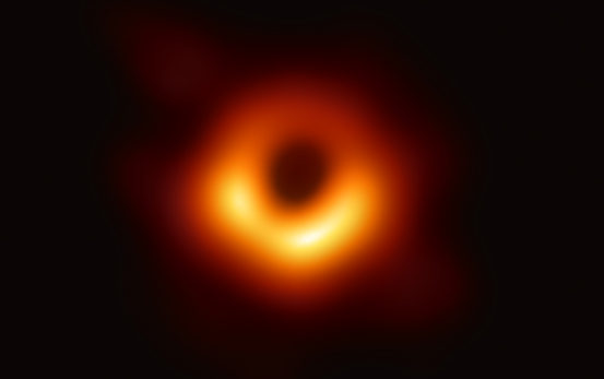 |
Cambridge Part III General Relativity diagram (Prof. Daniel Baumann): Geometric spacetime curvature, null cones, or orbits | [[Geodesic deviation and tidal forces]] |
 |
Cambridge Part III General Relativity diagram (Prof. Daniel Baumann): Geometric spacetime curvature, null cones, or orbits | [[Parallel transport and holonomy]] |
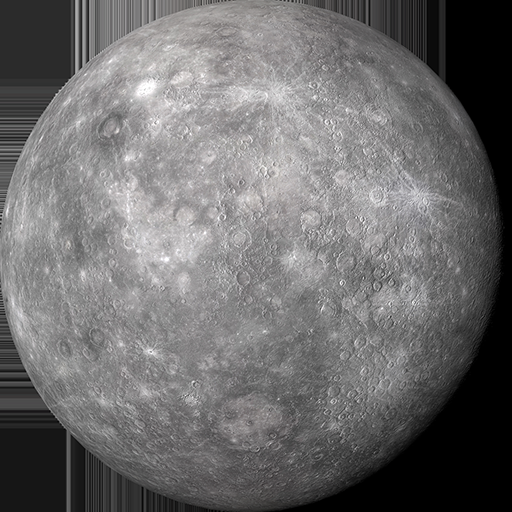 |
Cambridge Part III General Relativity diagram (Prof. Daniel Baumann): Geometric spacetime curvature, null cones, or orbits | [[Counting Riemann components]] |
 |
Cambridge Part III General Relativity diagram (Prof. Daniel Baumann): Geometric spacetime curvature, null cones, or orbits | [[Gravitational redshift and time dilation]] |
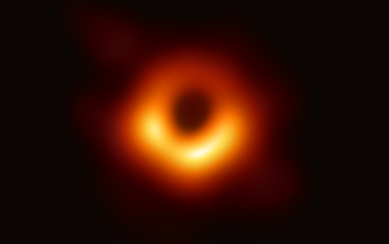 |
Cambridge Part III General Relativity diagram (Prof. Daniel Baumann): Geometric spacetime curvature, null cones, or orbits | [[Schwarzschild metric]] |
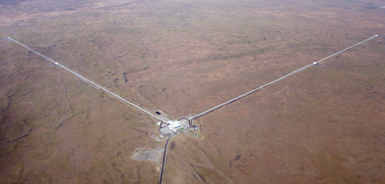 |
Cambridge Part III General Relativity diagram (Prof. Daniel Baumann): Geometric spacetime curvature, null cones, or orbits | [[Circular orbits in Schwarzschild]] |
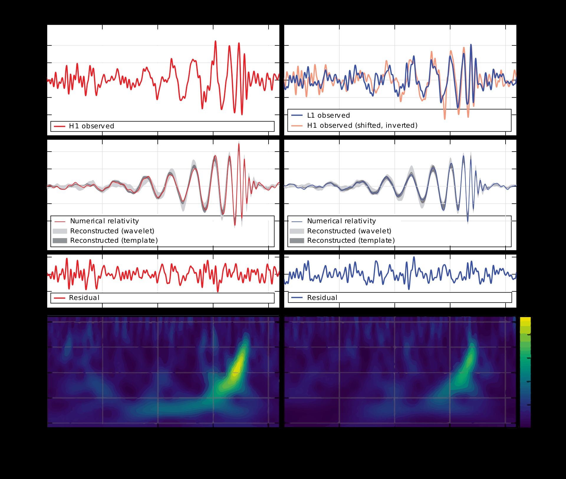 |
Cambridge Part III General Relativity diagram (Prof. Daniel Baumann): Geometric spacetime curvature, null cones, or orbits | [[Light deflection in Schwarzschild]] |
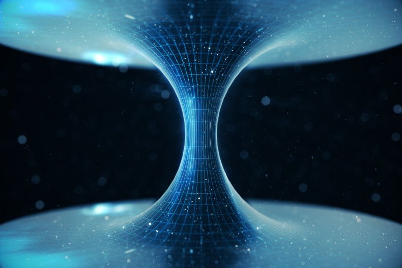 |
Cambridge Part III General Relativity diagram (Prof. Daniel Baumann): Geometric spacetime curvature, null cones, or orbits | [[Gravitational waves in General Relativity]] |
 |
Cambridge Part III General Relativity diagram (Prof. Daniel Baumann): Geometric spacetime curvature, null cones, or orbits | [[Cosmological perturbation theory in General Relativity]] |
 |
Question 1 Oral Exam Model Solution Card: Blackboard mathematical derivation and key physical result | [[Coordinate transformations and tensors]] |
 |
Question 2 Oral Exam Model Solution Card: Blackboard mathematical derivation and key physical result | [[Geodesic equation]] |
 |
Question 3 Oral Exam Model Solution Card: Blackboard mathematical derivation and key physical result | [[Killing vectors and symmetries]] |
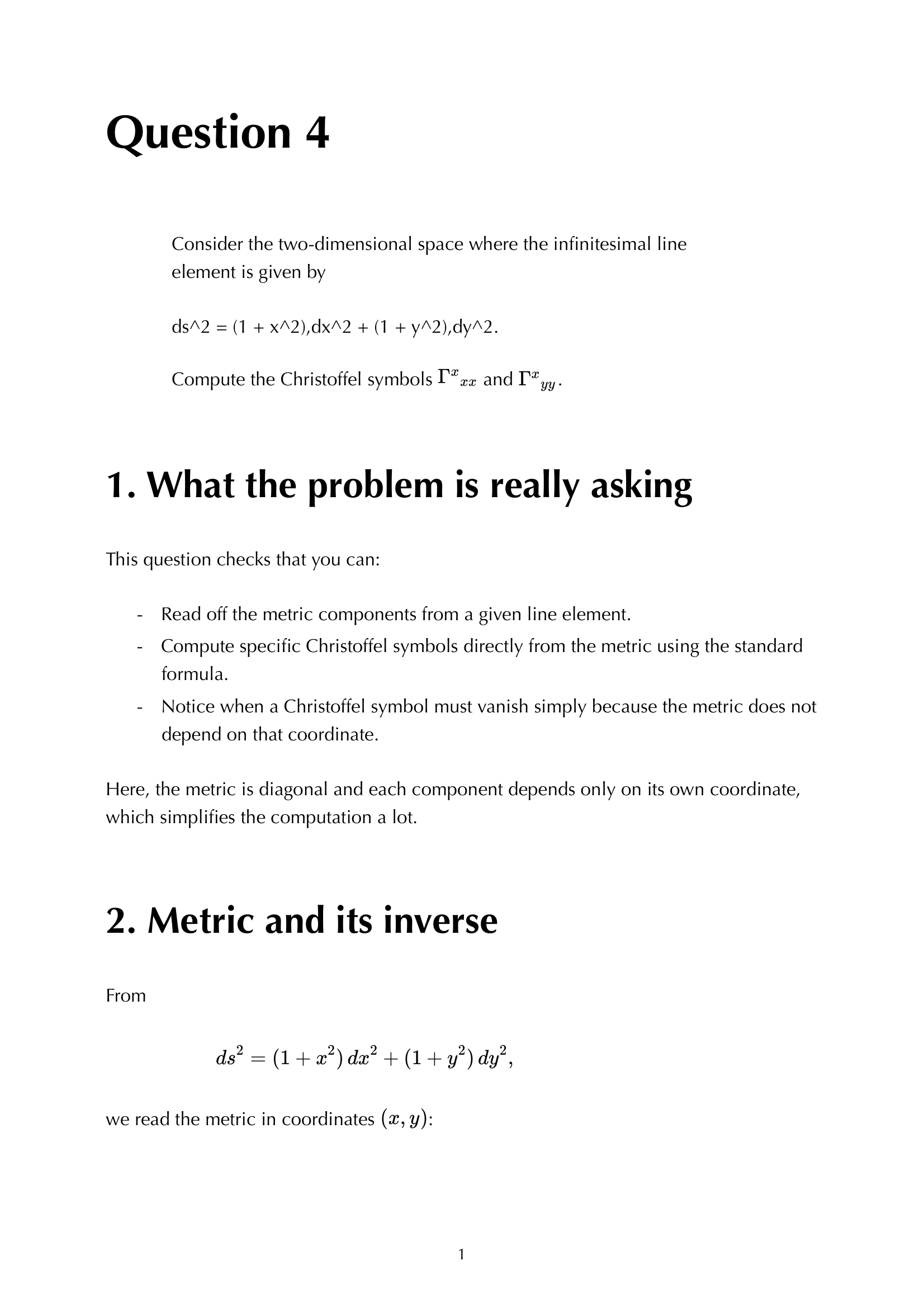 |
Question 4 Oral Exam Model Solution Card: Blackboard mathematical derivation and key physical result | [[Christoffel symbols]] |
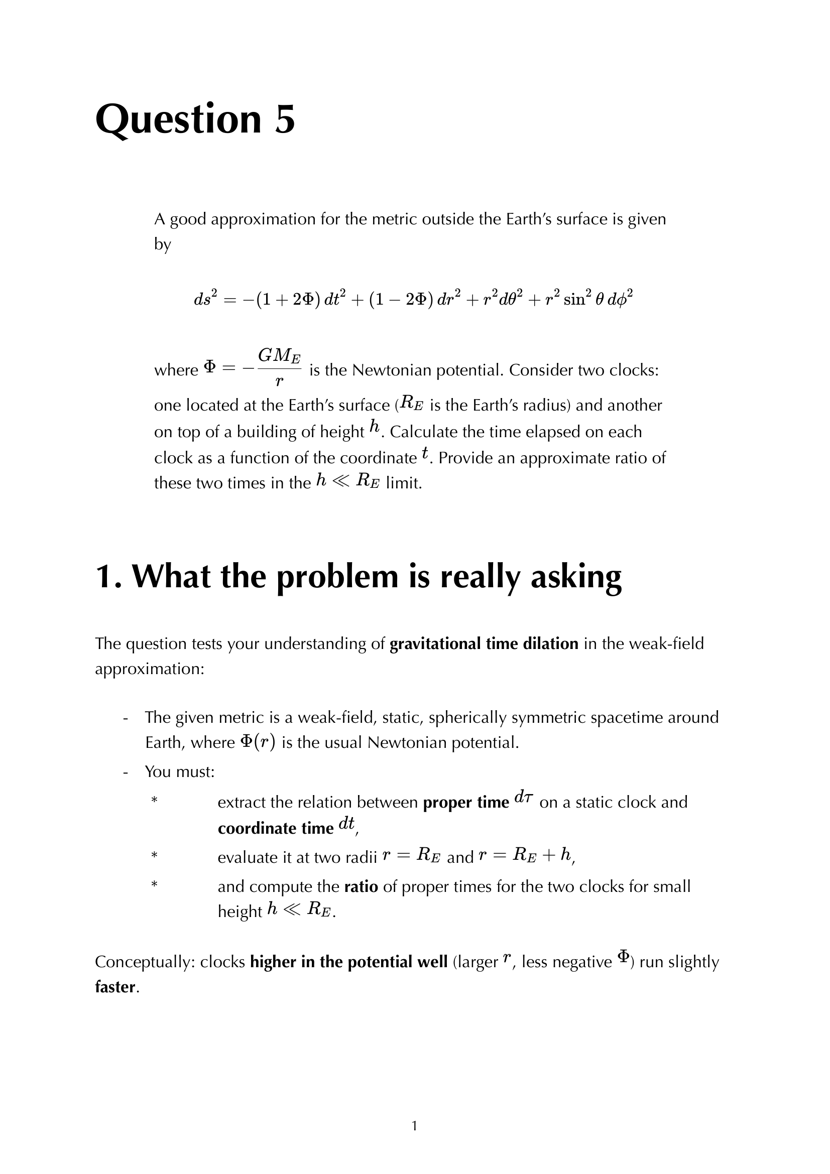 |
Question 5 Oral Exam Model Solution Card: Blackboard mathematical derivation and key physical result | [[Equivalence principle]] |
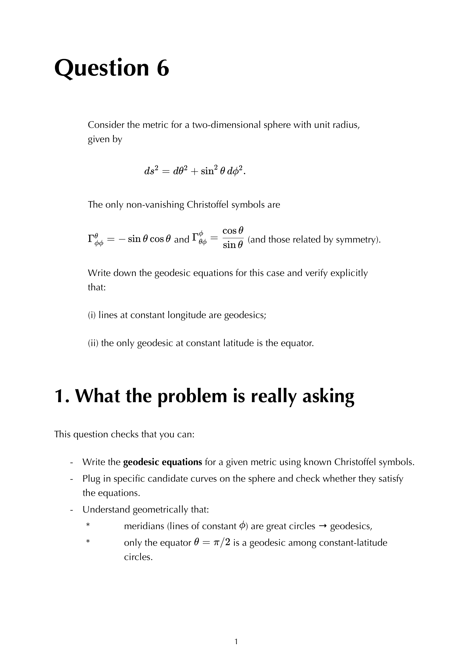 |
Question 6 Oral Exam Model Solution Card: Blackboard mathematical derivation and key physical result | [[Counting Riemann components]] |
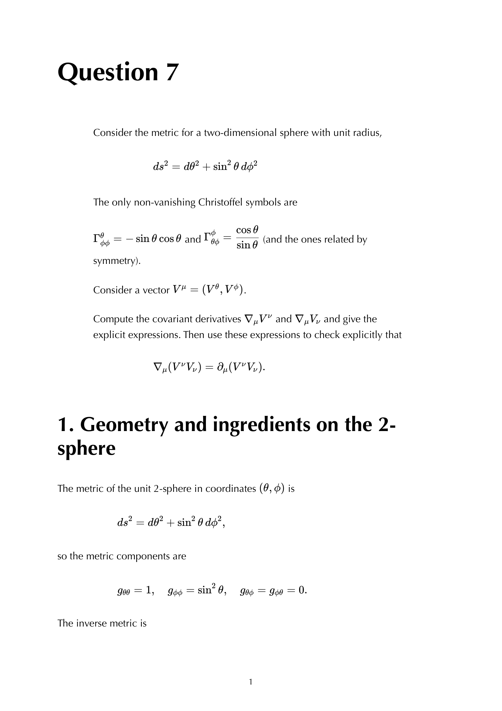 |
Question 7 Oral Exam Model Solution Card: Blackboard mathematical derivation and key physical result | [[Parallel transport and holonomy]] |
 |
Question 8 Oral Exam Model Solution Card: Blackboard mathematical derivation and key physical result | [[Bianchi identities]] |
 |
Question 9 Oral Exam Model Solution Card: Blackboard mathematical derivation and key physical result | [[Light deflection in Schwarzschild]] |
 |
Question 10 Oral Exam Model Solution Card: Blackboard mathematical derivation and key physical result | [[Schwarzschild metric]] |
 |
Question 11 Oral Exam Model Solution Card: Blackboard mathematical derivation and key physical result | [[Circular orbits in Schwarzschild]] |
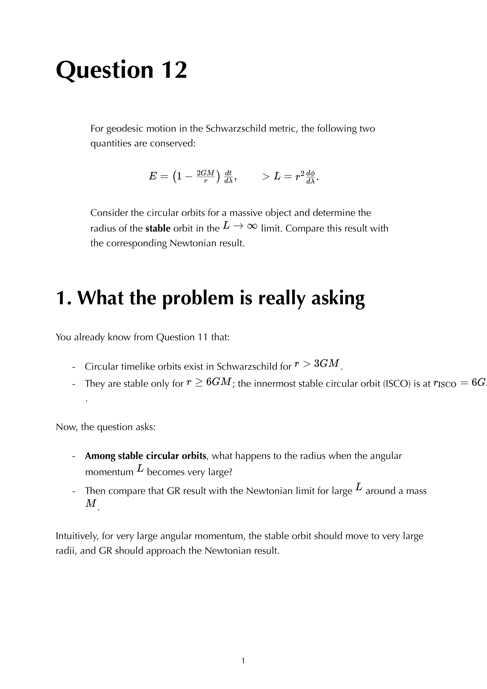 |
Question 12 Oral Exam Model Solution Card: Blackboard mathematical derivation and key physical result | [[Eddington-Finkelstein and Kruskal]] |
 |
Question 13 Oral Exam Model Solution Card: Blackboard mathematical derivation and key physical result | [[Light deflection in Schwarzschild]] |
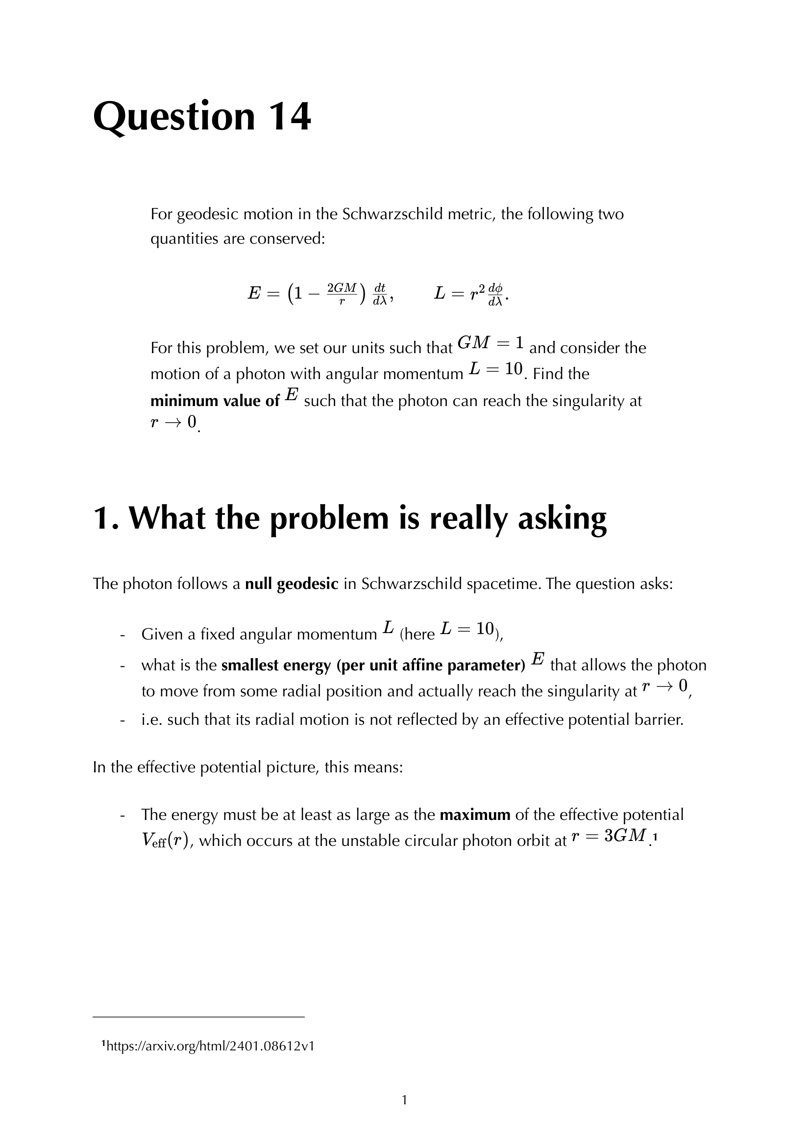 |
Question 14 Oral Exam Model Solution Card: Blackboard mathematical derivation and key physical result | [[Perihelion precession of Mercury]] |
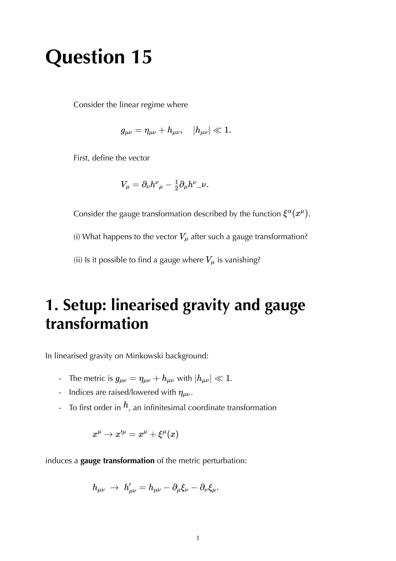 |
Question 15 Oral Exam Model Solution Card: Blackboard mathematical derivation and key physical result | [[Linearized gravity and gravitational waves]] |
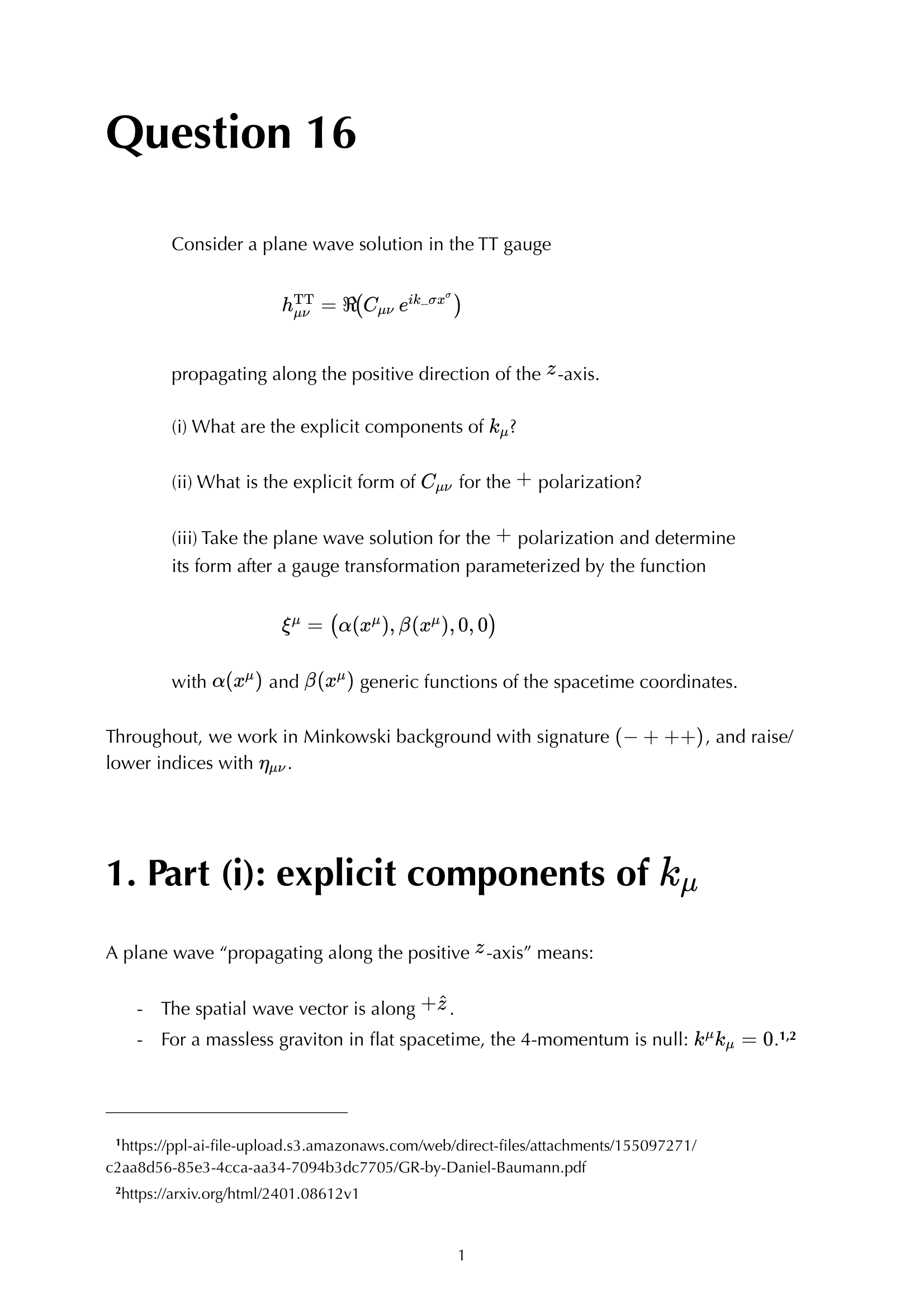 |
Question 16 Oral Exam Model Solution Card: Blackboard mathematical derivation and key physical result | [[Gravitational waves in General Relativity]] |
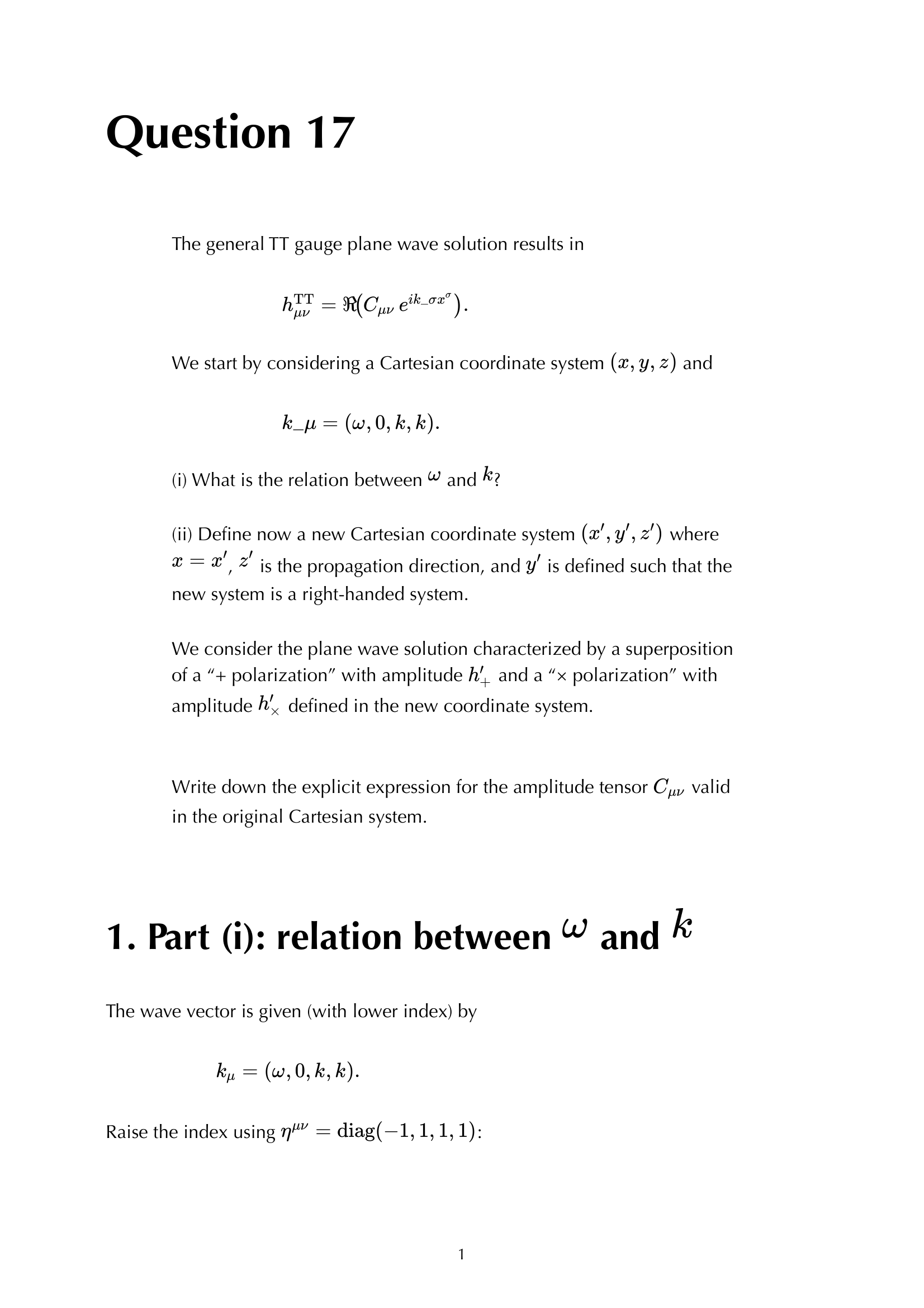 |
Question 17 Oral Exam Model Solution Card: Blackboard mathematical derivation and key physical result | [[Gravitational waves in General Relativity]] |
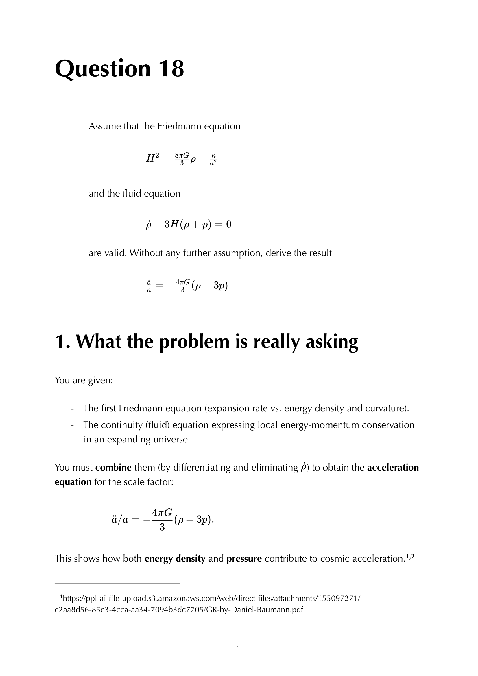 |
Question 18 Oral Exam Model Solution Card: Blackboard mathematical derivation and key physical result | [[Friedmann equations]] |
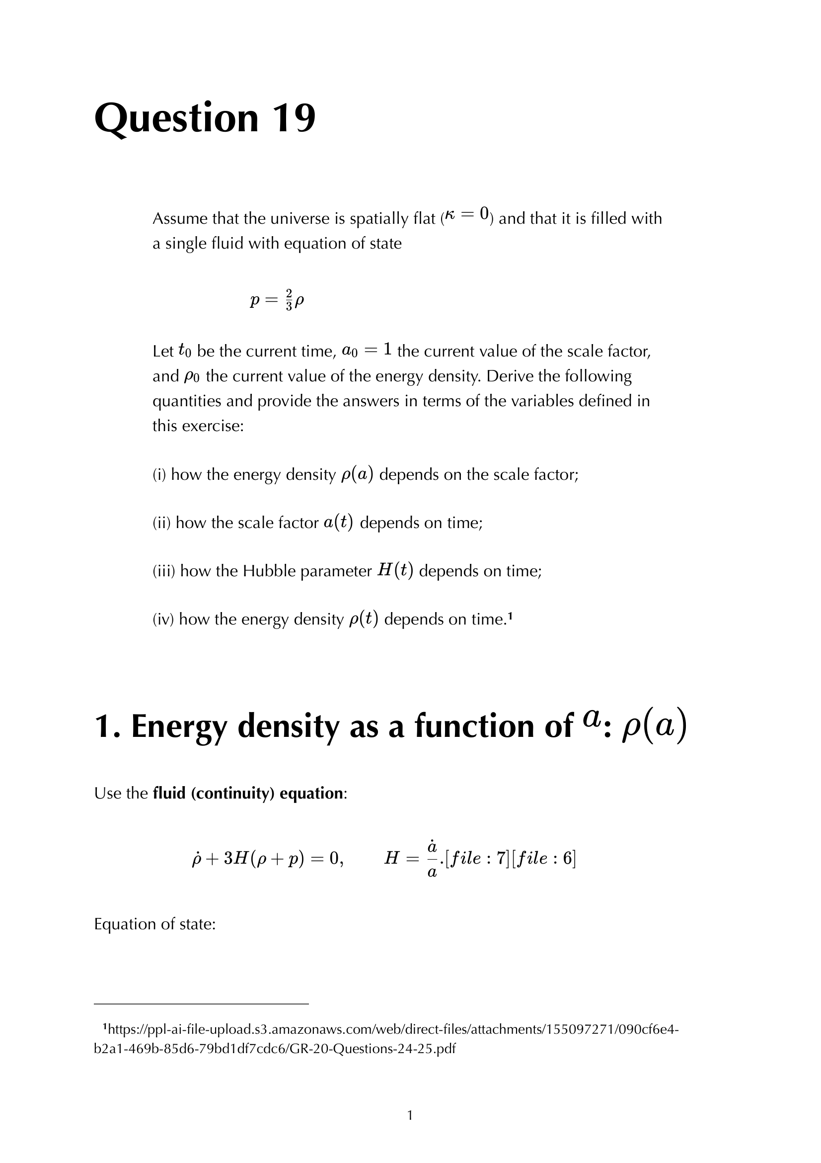 |
Question 19 Oral Exam Model Solution Card: Blackboard mathematical derivation and key physical result | [[Equation of state and density scaling]] |
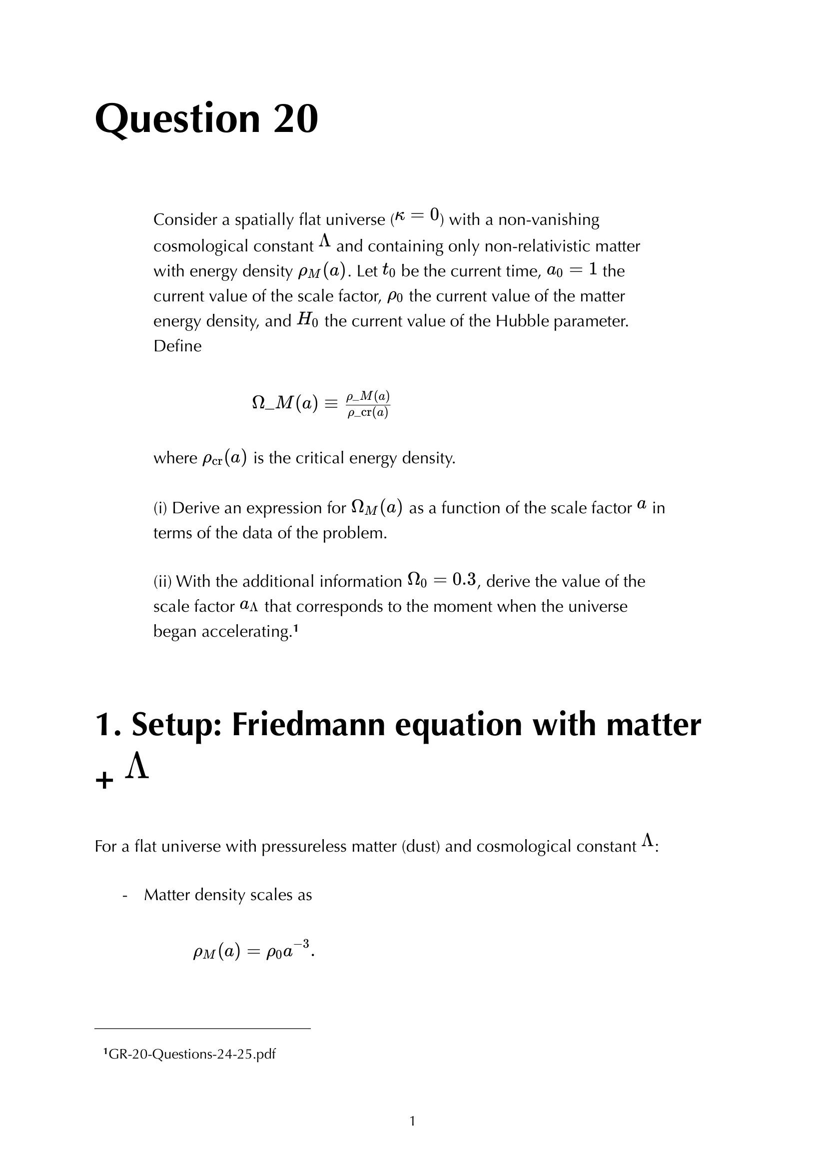 |
Question 20 Oral Exam Model Solution Card: Blackboard mathematical derivation and key physical result | [[Cosmological constant]] |
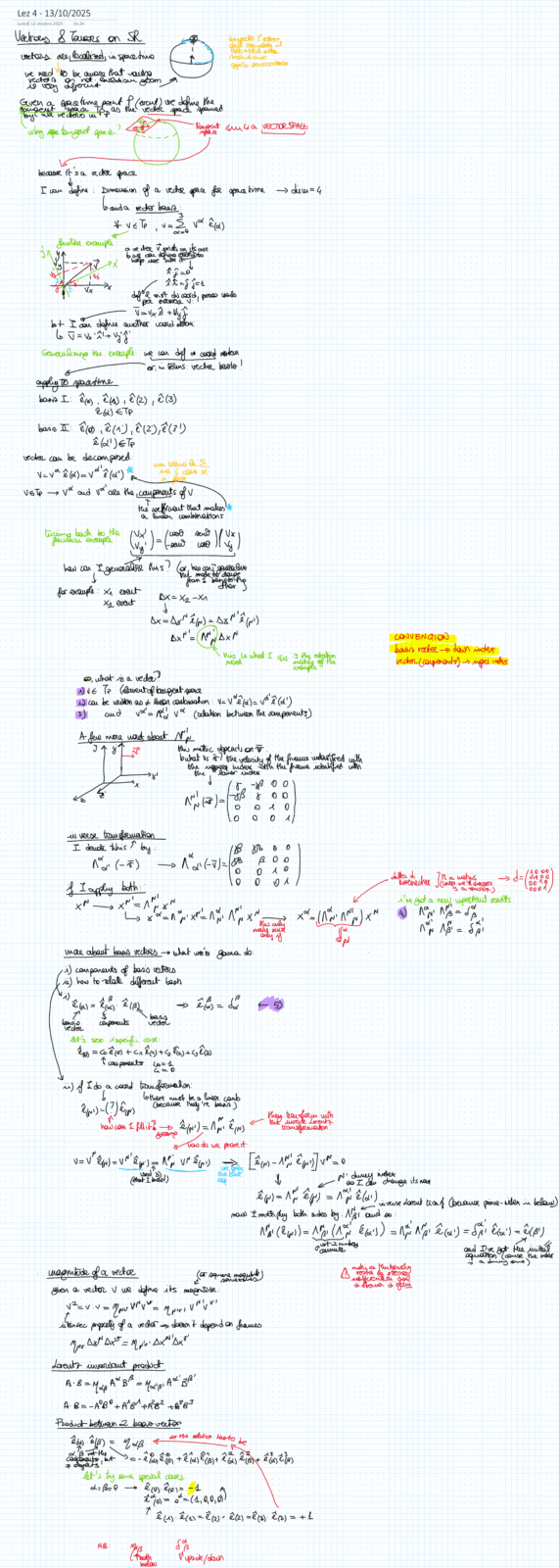 |
Padova University GR Lecture Blackboard Summary Sheet: Four-velocity, equivalence principle, energy-momentum tensor, or curvilinear coordinates | [[Equivalence principle]] |
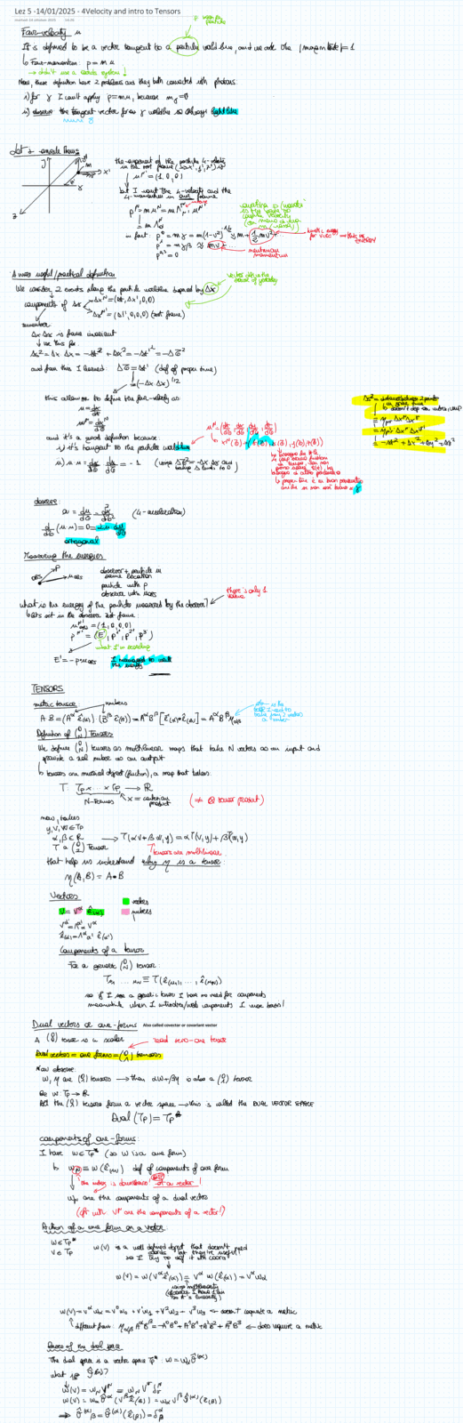 |
Padova University GR Lecture Blackboard Summary Sheet: Four-velocity, equivalence principle, energy-momentum tensor, or curvilinear coordinates | [[Four-velocity and four-momentum]] |
 |
Padova University GR Lecture Blackboard Summary Sheet: Four-velocity, equivalence principle, energy-momentum tensor, or curvilinear coordinates | [[Continuity equation]] |
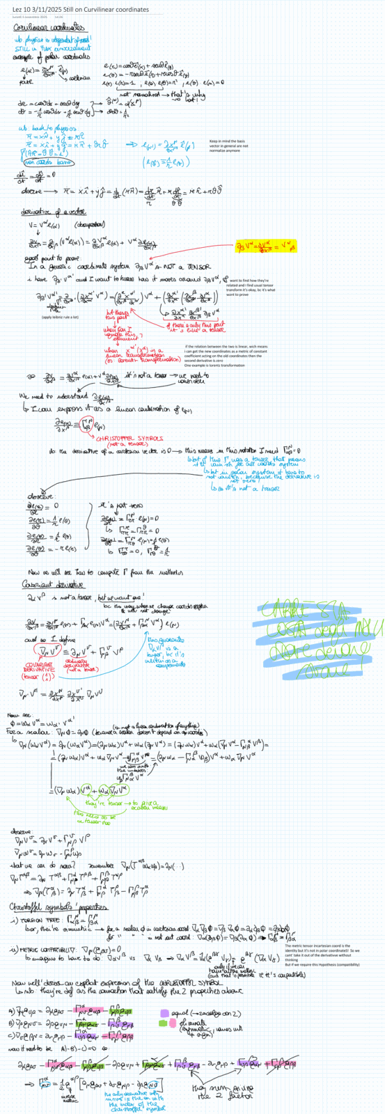 |
Padova University GR Lecture Blackboard Summary Sheet: Four-velocity, equivalence principle, energy-momentum tensor, or curvilinear coordinates | [[Coordinate transformations and tensors]] |
Wikipedia and arXiv sources
Every zettel in this map ends with a short sourced section: a definition quoted from Wikipedia (71 zettels) or from the abstract of an arXiv review (58 zettels), and, where a free figure exists, the credited lead figure of the Wikipedia article (Wikimedia Commons) or a figure from an openly licensed arXiv paper. The lecture-slide figures above are unchanged.
Professors Nicola Bartolo & Marco Peloso Oral Exam Defense Preparation Matrix
The oral examination for General Relativity draws directly from a published bank of 20 core mathematical problems. The following defense matrix details the exact question, starting formula, rigorous blackboard derivation steps, and key trap points for all 20 questions:
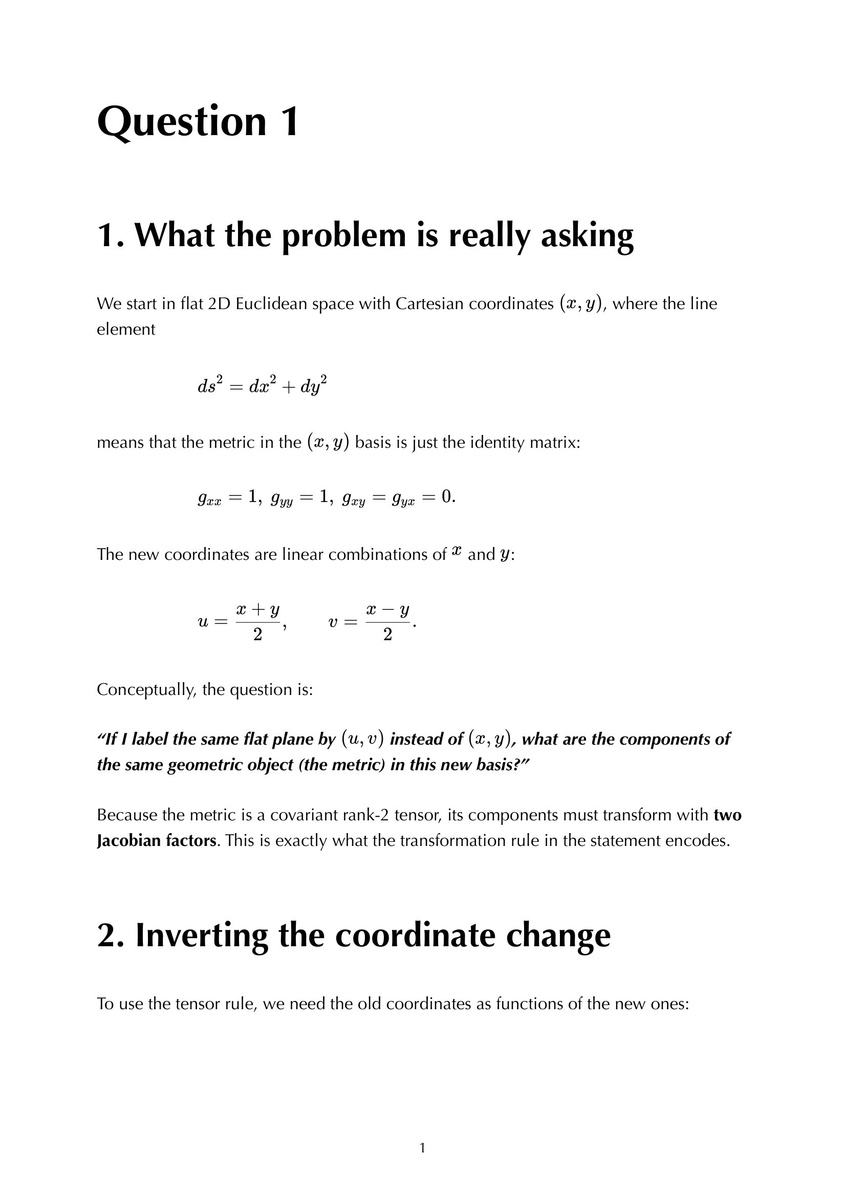
Question 01 - Flat 2D Euclidean Metric in Cartesian vs Polar Coordinates
- Official Exam Question & Figure Asset:
 - Starting Formula: \(ds^2 = dx^2 + dy^2\)
- Blackboard Derivation & Step-by-Step Proof:
- In Cartesian coordinates, $g_{ij} = \delta_{ij} = {\rm diag}(1,1)$, so $\partial_k g_{ij} = 0$ everywhere, implying all Christoffel symbols $\Gamma^k_{ij} = 0$.
- The geodesic equation $\ddot{x}^i + \Gamma^i_{jk}\dot{x}^j\dot{x}^k = 0$ simplifies to $\ddot{x}^i = 0$, whose solution is a straight line $x^i(\lambda) = v^i\lambda + x_0^i$.
- Transforming to polar coordinates $x = r\cos\phi, y = r\sin\phi$, the metric becomes $ds^2 = dr^2 + r^2 d\phi^2$. Here $\Gamma^r_{\phi\phi} = -r$ and $\Gamma^\phi_{r\phi} = 1/r$. The straight line is preserved physically, but non-zero Christoffel symbols represent coordinate acceleration (centrifugal and Coriolis forces).
- Professor Trap Points: Confusing non-zero Christoffel symbols with intrinsic curvature. Christoffel symbols depend on coordinate choice, Riemann tensor $R^i{}_{jkl} = 0$ proves the manifold is intrinsically flat!
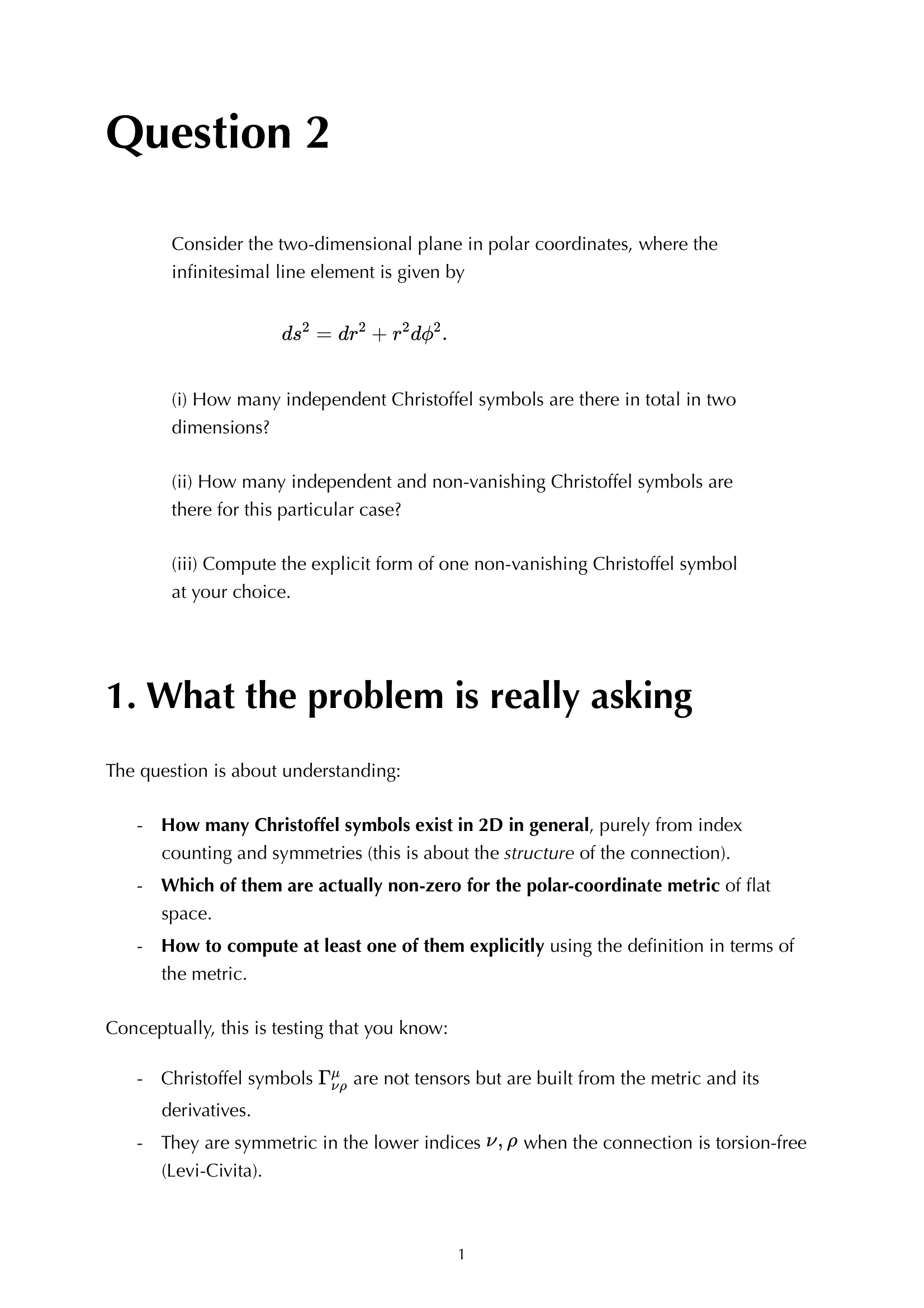
Question 02 - Geodesic Equations in 2D Polar Coordinates via Euler-Lagrange
- Official Exam Question & Figure Asset:
 - Starting Formula: \(L = \frac{1}{2} g_{\mu\nu} \dot{x}^\mu \dot{x}^\nu = \frac{1}{2}(\dot{r}^2 + r^2 \dot{\phi}^2)\)
- Blackboard Derivation & Step-by-Step Proof:
- Apply the Euler-Lagrange equations $\frac{d}{d\lambda}\left(\frac{\partial L}{\partial \dot{x}^i}\right) - \frac{\partial L}{\partial x^i} = 0$.
- For $r$: $\frac{\partial L}{\partial \dot{r}} = \dot{r}, \frac{\partial L}{\partial r} = r\dot{\phi}^2 \implies \ddot{r} - r\dot{\phi}^2 = 0$. Comparing with $\ddot{r} + \Gamma^r_{\mu\nu}\dot{x}^\mu\dot{x}^\nu = 0$, we read off $\Gamma^r_{\phi\phi} = -r$.
- For $\phi$: $\frac{\partial L}{\partial \phi} = 0$ (cyclic coordinate!), so conjugate momentum is conserved: $p_\phi = \frac{\partial L}{\partial \dot{\phi}} = r^2\dot{\phi} = J = {\rm const}$.
- Differentiating $r^2\dot{\phi} = {\rm const}$ gives $2r\dot{r}\dot{\phi} + r^2\ddot{\phi} = 0 \implies \ddot{\phi} + \frac{2}{r}\dot{r}\dot{\phi} = 0$, so $\Gamma^\phi_{r\phi} = \Gamma^\phi_{\phi r} = 1/r$.
- Professor Trap Points: Forgetting the symmetry factor 2 when matching $\Gamma^\phi_{r\phi}$ in $\ddot{x}^i + \Gamma^i_{jk}\dot{x}^j\dot{x}^k = 0$ because $\dot{r}\dot{\phi}$ appears twice!
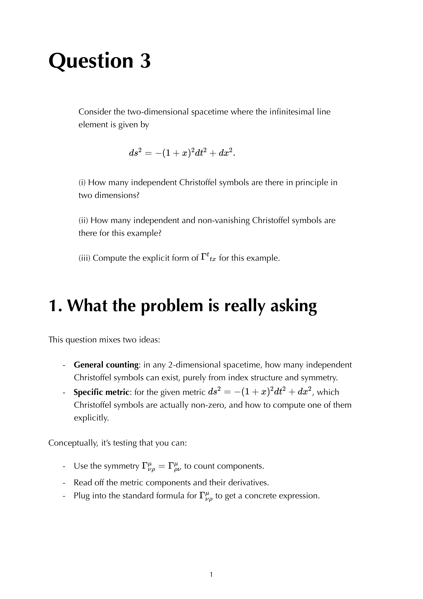
Question 03 - 2D Spacetime Symmetries and Killing Vectors
- Official Exam Question & Figure Asset:
 - Starting Formula: \(ds^2 = -(1+x^2)dt^2 + dx^2\)
- Blackboard Derivation & Step-by-Step Proof:
- The metric components are independent of time coordinate $t$: $\partial_t g_{\mu\nu} = 0$. Therefore, $\xi^\mu = \delta^\mu_t = (1, 0)$ is an exact timelike Killing vector.
- Check Killing’s equation: $\nabla_\mu \xi_\nu + \nabla_\nu \xi_\mu = \partial_\mu \xi_\nu + \partial_\nu \xi_\mu - 2\Gamma^\alpha_{\mu\nu}\xi_\alpha = 0$. Since $\xi_\nu = g_{\nu\mu}\xi^\mu = g_{\nu t} = (-(1+x^2), 0)$, all components satisfy the equation identically.
- Conserved quantity along any geodesic $u^\mu = dx^\mu/d\tau$: $E = -g_{\mu\nu}\xi^\mu u^\nu = (1+x^2)\frac{dt}{d\tau} = {\rm const}$. This represents energy per unit mass in static gravitational field.
- Professor Trap Points: Thinking $x$ provides a second Killing vector. The metric depends explicitly on $x$, so $\partial_x$ is NOT a Killing vector!
Question 04 - Christoffel Symbols and Riemann Curvature of 2D Metric
- Official Exam Question & Figure Asset:
 - Starting Formula: \(ds^2 = (1+x^2)dx^2 + (1+y^2)dy^2\)
- Blackboard Derivation & Step-by-Step Proof:
- Metric is diagonal: $g_{xx} = 1+x^2, g_{yy} = 1+y^2$, inverses $g^{xx} = (1+x^2)^{-1}, g^{yy} = (1+y^2)^{-1}$.
- Christoffels: $\Gamma^x_{xx} = \frac{1}{2}g^{xx}\partial_x g_{xx} = \frac{x}{1+x^2}$, $\Gamma^y_{yy} = \frac{y}{1+y^2}$. All cross components $\Gamma^x_{xy} = \Gamma^x_{yy} = \Gamma^y_{xx} = \Gamma^y_{xy} = 0$.
- Riemann tensor component: $R^x{}{yxy} = \partial_x \Gamma^x{yy} - \partial_y \Gamma^x_{xy} + \Gamma^x_{x\alpha}\Gamma^\alpha_{yy} - \Gamma^x_{y\alpha}\Gamma^\alpha_{xy} = 0 - 0 + 0 - 0 = 0$.
- In fact, all components of $R^i{}_{jkl} = 0$ identically! The coordinate transformations $X = \int \sqrt{1+x^2}dx$ and $Y = \int \sqrt{1+y^2}dy$ bring the metric directly to flat Cartesian form $ds^2 = dX^2 + dY^2$.
- Professor Trap Points: Performing tedious algebra on Riemann without recognizing that a diagonal metric whose components depend only on their own coordinates ($g_{11}(x^1), g_{22}(x^2)$) can always be transformed to flat space by simple 1D coordinate changes!
Question 05 - Weak-Field Metric Outside Earth and Clock Rates
- Official Exam Question & Figure Asset:
 - Starting Formula: \(ds^2 = -(1+2\Phi)dt^2 + (1-2\Phi)dr^2 + r^2 d\Omega^2, \quad \Phi = -\frac{GM}{r}\)
- Blackboard Derivation & Step-by-Step Proof:
- For a clock at rest at radius $r$: $dr = d\theta = d\phi = 0$, so proper time is $d\tau = \sqrt{-ds^2} = \sqrt{1 + 2\Phi}\,dt \approx (1 + \Phi)\,dt$.
- Comparing two stationary clocks at radii $r_1$ and $r_2$ ($r_2 > r_1$): $\frac{d\tau_2}{d\tau_1} = \frac{1 + \Phi(r_2)}{1 + \Phi(r_1)} \approx 1 + [\Phi(r_2) - \Phi(r_1)] = 1 - \frac{GM}{r_2} + \frac{GM}{r_1} > 1$.
- A clock higher up in the gravitational potential runs faster than a clock on Earth’s surface. For GPS satellites ($r_2 \approx 26,600$ km vs $r_1 \approx 6,370$ km), the gravitational blue-shift advances clocks by $\sim +45.9\,\mu$s/day (partially counteracted by special relativistic time dilation $\sim -7.2\,\mu$s/day, net $+38.7\,\mu$s/day).
- Professor Trap Points: Forgetting that $\Phi < 0$ for attractive Newtonian gravity, which flips the sign if not tracked carefully!
Question 06 - Christoffel and Curvature of Unit 2-Sphere $S^2$
- Official Exam Question & Figure Asset:
 - Starting Formula: \(ds^2 = d\theta^2 + \sin^2\theta d\phi^2\)
- Blackboard Derivation & Step-by-Step Proof:
- Metric: $g_{\theta\theta} = 1, g_{\phi\phi} = \sin^2\theta$. Non-zero Christoffel symbols: $\Gamma^\theta_{\phi\phi} = -\sin\theta\cos\theta$, $\Gamma^\phi_{\theta\phi} = \Gamma^\phi_{\phi\theta} = \cot\theta$.
- Riemann curvature: $R^\theta{}{\phi\theta\phi} = \partial\theta\Gamma^\theta_{\phi\phi} - \partial_\phi\Gamma^\theta_{\theta\phi} + \Gamma^\theta_{\theta\lambda}\Gamma^\lambda_{\phi\phi} - \Gamma^\theta_{\phi\lambda}\Gamma^\lambda_{\theta\phi} = -(\cos^2\theta - \sin^2\theta) - (-\sin\theta\cos\theta)(\cot\theta) = \sin^2\theta$.
- Ricci tensor: $R_{\theta\theta} = R^\phi{}{\theta\phi\theta} = 1$, $R{\phi\phi} = R^\theta{}_{\phi\theta\phi} = \sin^2\theta$.
- Ricci scalar: $R = g^{ij}R_{ij} = 1(1) + \frac{1}{\sin^2\theta}(\sin^2\theta) = 1 + 1 = 2$. For sphere of radius $a$, $R = 2/a^2$.
- Professor Trap Points: Forgetting that $R_{\phi\phi} = \sin^2\theta$, so the contracted scalar $R = g^{\theta\theta}R_{\theta\theta} + g^{\phi\phi}R_{\phi\phi} = 1 + 1 = 2$, NOT 1!
Question 07 - Parallel Transport on 2-Sphere and Holonomy Angle
- Official Exam Question & Figure Asset:
 - Starting Formula: \(\nabla_{\dot{\gamma}} V^\mu = 0 \implies \frac{dV^\mu}{d\lambda} + \Gamma^\mu_{\alpha\beta} V^\alpha \frac{dx^\beta}{d\lambda} = 0\)
- Blackboard Derivation & Step-by-Step Proof:
- Consider parallel transporting a vector along a latitude circle $\theta = \theta_0$ parameterized by $\phi \in [0, 2\pi]$. Here $\dot{\theta} = 0, \dot{\phi} = 1$.
- Components: $\frac{dV^\theta}{d\phi} + \Gamma^\theta_{\phi\phi} V^\phi = 0 \implies \frac{dV^\theta}{d\phi} - \sin\theta_0\cos\theta_0 V^\phi = 0$.
- Second component: $\frac{dV^\phi}{d\phi} + \Gamma^\phi_{\theta\phi} V^\theta = 0 \implies \frac{dV^\phi}{d\phi} + \cot\theta_0 V^\theta = 0$.
- Differentiate again to get a harmonic oscillator: $\frac{d^2 V^\theta}{d\phi^2} + \cos^2\theta_0 V^\theta = 0$. Solution: $V^\theta(\phi) = V_0 \cos(\phi\cos\theta_0)$.
- After complete circuit $\Delta\phi = 2\pi$, the vector has rotated by phase angle $\alpha = 2\pi\cos\theta_0$. The deficit angle (holonomy) is $\Delta\psi = 2\pi - \alpha = 2\pi(1 - \cos\theta_0) = \iint K dA$, which is exactly the solid angle enclosed by the loop (Gauss-Bonnet theorem)!
- Professor Trap Points: Stating that the vector returns unchanged. On a curved manifold, parallel transport around a closed loop rotates the vector by an angle equal to the integrated curvature!
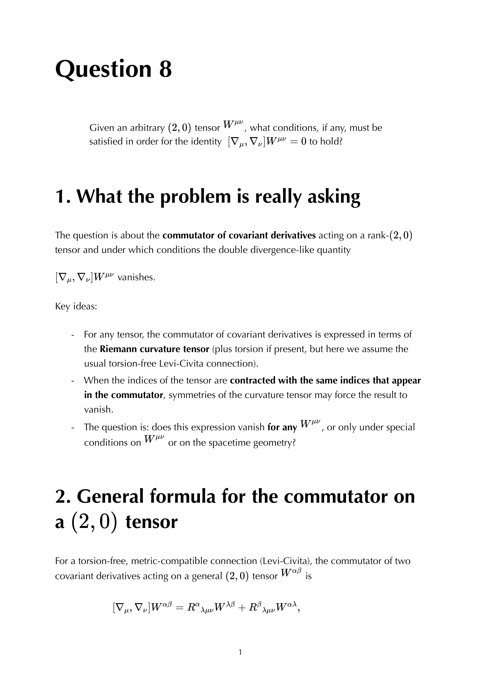
Question 08 - Commutator of Covariant Derivatives and Bianchi Identity
- Official Exam Question & Figure Asset:
 - Starting Formula: \([\nabla_\mu, \nabla_\nu] W^{\alpha\beta} = R^\alpha{}_{\lambda\mu\nu} W^{\lambda\beta} + R^\beta{}_{\lambda\mu\nu} W^{\alpha\lambda}\)
- Blackboard Derivation & Step-by-Step Proof:
- For an arbitrary $(2,0)$ tensor $W^{\mu\nu}$, the commutator of covariant derivatives generates Riemann curvature terms for each index.
- Contracting $\alpha = \mu$ and $\beta = \nu$: $[\nabla_\mu, \nabla_\nu] W^{\mu\nu} = R^\mu{}{\lambda\mu\nu} W^{\lambda\nu} + R^\nu{}{\lambda\mu\nu} W^{\mu\lambda} = R_{\lambda\nu} W^{\lambda\nu} - R_{\lambda\mu} W^{\mu\lambda}$.
- If $W^{\mu\nu}$ is symmetric ($W^{\mu\nu} = W^{\nu\mu}$), then $R_{\mu\nu} W^{\mu\nu} - R_{\nu\mu} W^{\nu\mu} = 0$ identically because $R_{\mu\nu}$ is symmetric!
- Therefore, the condition for $[\nabla_\mu, \nabla_\nu] W^{\mu\nu} = 0$ is that $W^{\mu\nu}$ is a symmetric tensor. This is the geometric foundation for the divergence-free Einstein tensor $\nabla_\mu G^{\mu\nu} = 0$.
- Professor Trap Points: Assuming $[\nabla_\mu, \nabla_\nu] W^{\mu\nu} = 0$ holds for any tensor. If $W^{\mu\nu}$ has an antisymmetric part $A^{\mu\nu}$, the contraction yields $2 R_{\mu\nu} A^{\mu\nu} \ne 0$!
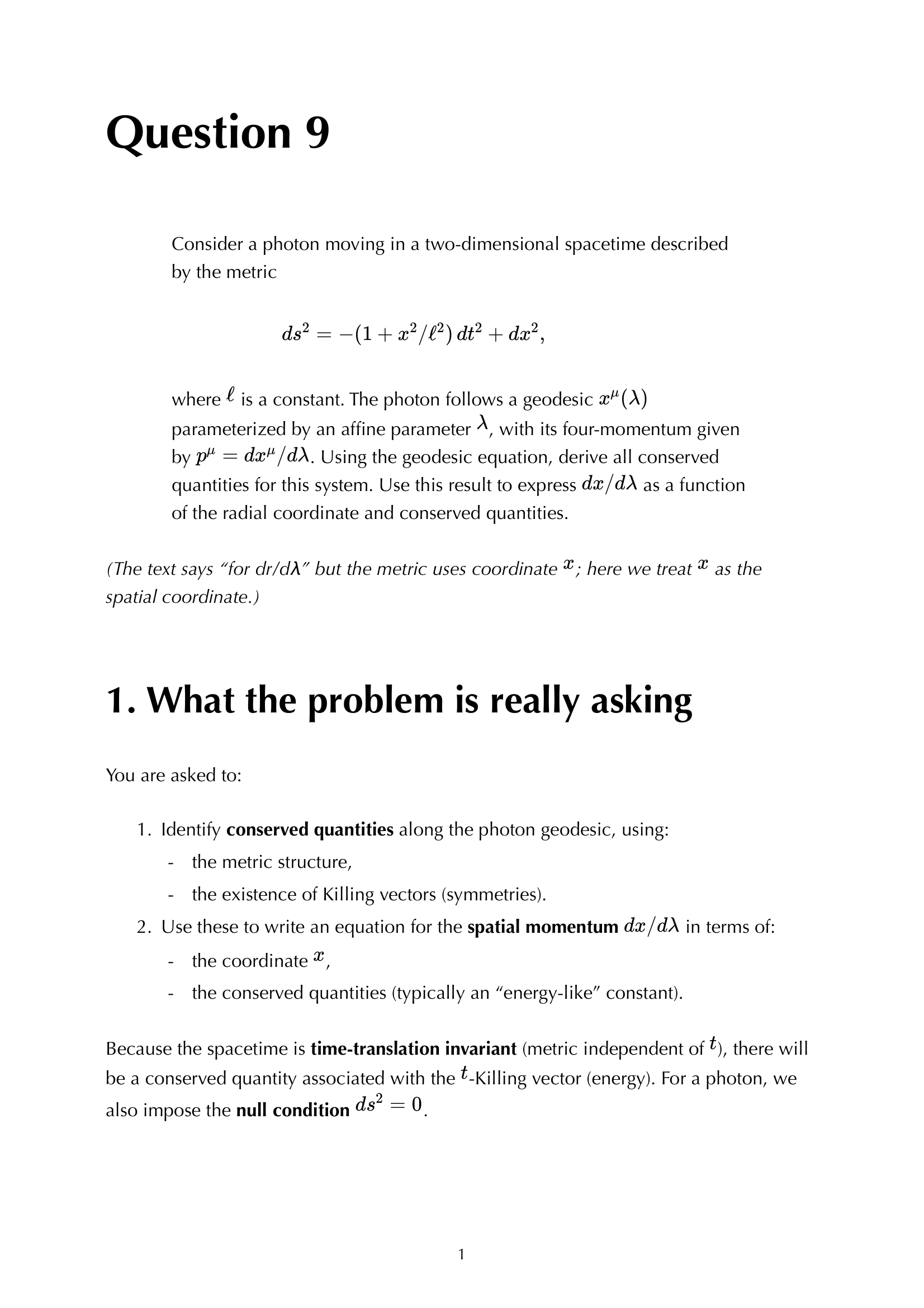
Question 09 - Photon Trajectory and Coordinate Speed of Light in 2D
- Official Exam Question & Figure Asset:
 - Starting Formula: \(ds^2 = -(1 + x^2/\ell^2)dt^2 + dx^2 = 0\)
- Blackboard Derivation & Step-by-Step Proof:
- Photons travel along null geodesics ($ds^2 = 0$). Setting $ds^2 = 0$ gives $\left(\frac{dx}{dt}\right)^2 = 1 + \frac{x^2}{\ell^2}$.
- The coordinate velocity of light is $v(x) = \frac{dx}{dt} = \pm \sqrt{1 + x^2/\ell^2}$. Unlike in special relativity where $v=c=1$ is constant, coordinate speed depends on location!
- Integrating from $x=0$ at $t=0$: $\int_0^x \frac{dx’}{\sqrt{1 + x’^2/\ell^2}} = \int_0^t dt’ \implies \ell\operatorname{arcsinh}(x/\ell) = t \implies x(t) = \ell\sinh(t/\ell)$.
- Proper speed measured by a local stationary observer with orthonormal basis $\hat{e}0 = (1+x^2/\ell^2)^{-1/2}\partial_t, \hat{e}_1 = \partial_x$ is $v{\rm local} = \frac{dx^{\hat{1}}}{dt^{\hat{0}}} = 1 = c$ everywhere.
- Professor Trap Points: Confusing coordinate velocity $\frac{dx}{dt}$ with locally measured physical velocity $\frac{dx^{\hat{1}}}{dt^{\hat{0}}}$. Local velocity of light is ALWAYS $c$!
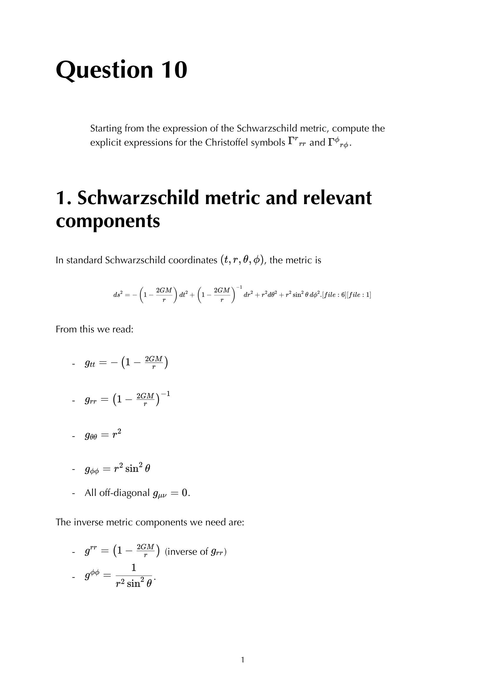
Question 10 - Schwarzschild Christoffel Symbols $\Gamma^r_{rr}$ and $\Gamma^r_{\phi\phi}$
- Official Exam Question & Figure Asset:
 - Starting Formula: \(ds^2 = -\left(1 - \frac{2GM}{r}\right)dt^2 + \left(1 - \frac{2GM}{r}\right)^{-1}dr^2 + r^2(d\theta^2 + \sin^2\theta d\phi^2)\)
- Blackboard Derivation & Step-by-Step Proof:
- Let $f(r) = 1 - \frac{2GM}{r}$. Then $g_{rr} = f(r)^{-1}$, so $\partial_r g_{rr} = -f(r)^{-2}f’(r) = -f^{-2}\frac{2GM}{r^2}$.
- Christoffel symbol: $\Gamma^r_{rr} = \frac{1}{2}g^{rr}\partial_r g_{rr} = \frac{1}{2}f \left(-f^{-2}\frac{2GM}{r^2}\right) = -\frac{GM}{r^2 f(r)} = -\frac{GM}{r(r - 2GM)}$.
- For $\Gamma^r_{\phi\phi}$: $g_{\phi\phi} = r^2\sin^2\theta$, so $\partial_r g_{\phi\phi} = 2r\sin^2\theta$.
- Formula: $\Gamma^r_{\phi\phi} = -\frac{1}{2}g^{rr}\partial_r g_{\phi\phi} = -\frac{1}{2}f(r)(2r\sin^2\theta) = -r\left(1 - \frac{2GM}{r}\right)\sin^2\theta$. In the equatorial plane $\theta = \pi/2$, $\Gamma^r_{\phi\phi} = -(r - 2GM)$.
- Professor Trap Points: Missing the negative sign in $\Gamma^r_{\phi\phi} = -\frac{1}{2}g^{rr}\partial_r g_{\phi\phi}$ which comes from the Euler-Lagrange kinetic term $-\frac{\partial L}{\partial r}$!
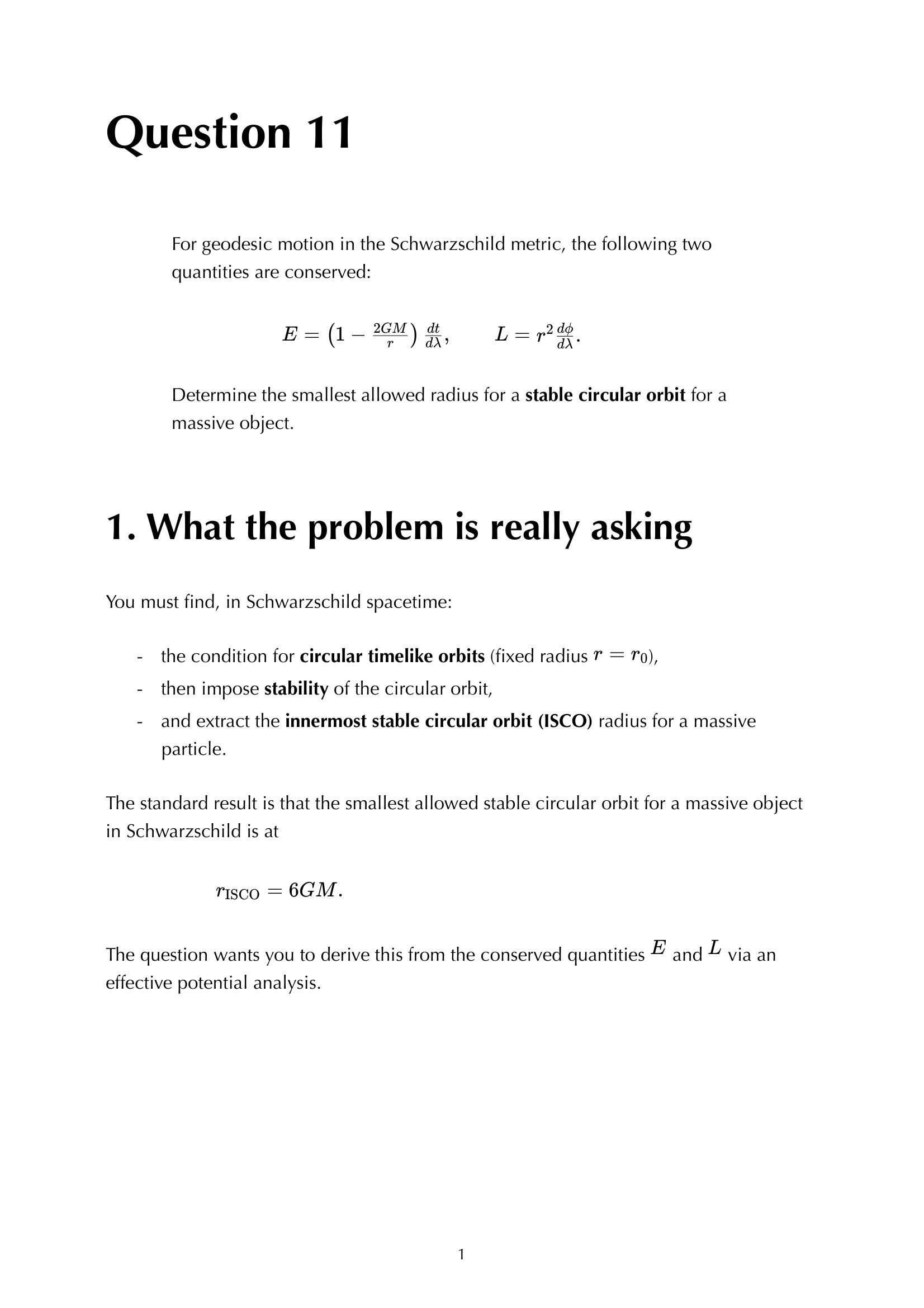
Question 11 - Effective Potential and Circular Orbits in Schwarzschild
- Official Exam Question & Figure Asset:
 - Starting Formula: \(\frac{1}{2}\left(\frac{dr}{d\lambda}\right)^2 + V_{\rm eff}(r) = \frac{E^2 - 1}{2}, \quad V_{\rm eff}(r) = -\frac{GM}{r} + \frac{L^2}{2r^2} - \frac{GML^2}{r^3}\)
- Blackboard Derivation & Step-by-Step Proof:
- Circular orbits require $\frac{dr}{d\lambda} = 0$ and $\frac{dV_{\rm eff}}{dr} = 0$.
- Derivative: $\frac{dV_{\rm eff}}{dr} = \frac{GM}{r^2} - \frac{L^2}{r^3} + \frac{3GML^2}{r^4} = 0 \implies GM r^2 - L^2 r + 3GM L^2 = 0$.
- Solving quadratic for $r$: $r = \frac{L^2 \pm \sqrt{L^4 - 12 G^2 M^2 L^2}}{2GM} = \frac{L^2}{2GM}\left[1 \pm \sqrt{1 - \frac{12 G^2 M^2}{L^2}}\right]$.
- Real solutions exist only if discriminant $\ge 0 \implies L^2 \ge 12 G^2 M^2$. At $L^2 = 12 G^2 M^2$, both roots merge at $r = \frac{12 G^2 M^2}{2GM} = 6GM$.
- Stability requires $\frac{d^2 V_{\rm eff}}{dr^2} > 0$. The outer root is stable, the inner root is unstable. At $r = 6GM$, $\frac{d^2 V_{\rm eff}}{dr^2} = 0$, defining the Innermost Stable Circular Orbit (ISCO) at $r_{\rm ISCO} = 6GM = 3 R_s$.
- Professor Trap Points: Forgetting the relativistic term $-GML^2/r^3$ in the effective potential, which has no Newtonian analog and is responsible for orbital instability and ISCO!
Question 12 - Radial Free-Fall Infall Proper Time vs Coordinate Time
- Official Exam Question & Figure Asset:
 - Starting Formula: \(\left(\frac{dr}{d\tau}\right)^2 = \frac{2GM}{r} \quad \text{(released from rest at } r_0 \to \infty \text{)}\)
- Blackboard Derivation & Step-by-Step Proof:
- For particle released from rest at $r_0$, energy parameter is $E = \sqrt{1 - 2GM/r_0} \le 1$. Take $r_0 \gg 2GM$ so $E \approx 1$.
- Radial equation: $\frac{dr}{d\tau} = -\sqrt{\frac{2GM}{r}} \implies \sqrt{r}\,dr = -\sqrt{2GM}\,d\tau$.
- Integrate from $r_0$ to $r=0$: $\tau = \int_0^{r_0} \sqrt{\frac{r}{2GM}}\,dr = \frac{2}{3\sqrt{2GM}} r_0^{3/2} = \frac{4}{3}\frac{GM}{c^3}\left(\frac{r_0}{2GM}\right)^{3/2}$. This is finite!
- Coordinate time: $\frac{dt}{dr} = \frac{dt/d\tau}{dr/d\tau} = -\frac{E/(1 - 2GM/r)}{\sqrt{2GM/r}}$. Near $r \to 2GM$, the integrand diverges as $\sim \frac{2GM}{r - 2GM}$.
- Integration yields $t(r) \sim -2GM \ln(r - 2GM) \to +\infty$ as $r \to 2GM$. The infalling astronaut crosses the horizon in finite proper time $\tau$, but an outside observer sees them redshift and freeze at the horizon as $t \to \infty$.
- Professor Trap Points: Stating that the astronaut cannot cross the horizon because $t \to \infty$. Coordinate time $t$ is pathological at $r = 2GM$, proper time $\tau$ is the physical invariant!
Question 13 - Photon Sphere and Weak Light Deflection
- Official Exam Question & Figure Asset:
 - Starting Formula: \(\left(\frac{dr}{d\lambda}\right)^2 + V_{\rm eff}^{\rm null}(r) = \frac{1}{b^2}, \quad V_{\rm eff}^{\rm null}(r) = \frac{1}{r^2}\left(1 - \frac{2GM}{r}\right)\)
- Blackboard Derivation & Step-by-Step Proof:
- For null geodesics, circular photon orbit requires $\frac{dV_{\rm eff}^{\rm null}}{dr} = 0$: $-\frac{2}{r^3} + \frac{6GM}{r^4} = 0 \implies r_{\rm ph} = 3GM = 1.5 R_s$.
- The critical impact parameter for photon capture is $b_{\rm crit} = \frac{1}{\sqrt{V_{\rm eff}(3GM)}} = 3\sqrt{3}GM \approx 5.196 GM$.
- For weak deflection ($b \gg b_{\rm crit}$), rewrite orbit in $u = 1/r$: $\frac{d^2 u}{d\phi^2} + u = 3GM u^2$.
- Zeroth order (straight line): $u_0(\phi) = \frac{\cos\phi}{b}$. First-order perturbation: $u_1(\phi) = \frac{GM}{b^2}(1 + \sin^2\phi)$.
- Total deflection angle: $\Delta\phi = 2\lvert u_1(\pi/2)\rvert b = \frac{4GM}{c^2 b}$. For the Sun ($M = M_\odot, b = R_\odot$), $\Delta\phi = 1.751$ arcseconds, confirming Dyson, Eddington & Davidson (1919).
- Professor Trap Points: Mixing up the Newtonian deflection $\Delta\phi_{\rm Newton} = \frac{2GM}{c^2 b}$ with Einstein’s GR deflection $\frac{4GM}{c^2 b}$. Space curvature doubles the Newtonian prediction!
Question 14 - Perihelion Precession of Mercury
- Official Exam Question & Figure Asset:
 - Starting Formula: \(\frac{d^2 u}{d\phi^2} + u = \frac{GM}{L^2} + 3GM u^2\)
- Blackboard Derivation & Step-by-Step Proof:
- In Newtonian gravity, $\frac{d^2 u}{d\phi^2} + u = \frac{GM}{L^2}$ gives unclosed Keplerian ellipse $u_0(\phi) = \frac{1}{p}(1 + e\cos\phi)$, where $p = a(1-e^2)$.
- Insert $u_0$ into the relativistic correction: $3GM u^2 \approx 3GM \frac{1}{p^2}(1 + 2e\cos\phi + e^2\cos^2\phi)$. The resonance term proportional to $\cos\phi$ drives precession.
- Equation for first-order perturbation $u_1$: $\frac{d^2 u_1}{d\phi^2} + u_1 = \frac{6GM e}{p^2}\cos\phi$.
- Particular solution of driven oscillator: $u_1(\phi) = \frac{3GM e}{p^2}\phi\sin\phi$.
- Total solution: $u(\phi) = \frac{1}{p}[1 + e(\cos\phi + \epsilon\phi\sin\phi)] \approx \frac{1}{p}[1 + e\cos(\phi(1 - \epsilon))]$, where $\epsilon = \frac{3GM}{p}$.
- The perihelion occurs when argument equals $2\pi$: $\phi(1 - \epsilon) = 2\pi \implies \phi \approx 2\pi(1 + \epsilon) = 2\pi + \Delta\phi$.
- Precession per orbit: $\Delta\phi = 2\pi\epsilon = \frac{6\pi GM}{c^2 a(1-e^2)}$. For Mercury ($a = 0.387$ AU, $e=0.206$, period 88 days), this gives exactly $42.98’’/$century!
- Professor Trap Points: Dropping the factor of 3 in the relativistic term $3GM u^2$ or failing to identify the secular resonance term $\phi\sin\phi$!
Question 15 - Linearized Gravity and Gauge Invariance
- Official Exam Question & Figure Asset:
 - Starting Formula: \(g_{\mu\nu} = \eta_{\mu\nu} + h_{\mu\nu}, \quad \lvert h_{\mu\nu}\rvert \ll 1\)
- Blackboard Derivation & Step-by-Step Proof:
- Under coordinate transformation $x^\mu \to x’^\mu = x^\mu + \xi^\mu(x)$ with $\lvert\partial_\mu \xi_\nu\rvert \sim \mathcal{O}(h)$, the metric perturbation transforms as: $h_{\mu\nu} \to h’{\mu\nu} = h{\mu\nu} - \partial_\mu \xi_\nu - \partial_\nu \xi_\mu$.
- Define trace-reversed metric perturbation: $\bar{h}{\mu\nu} = h{\mu\nu} - \frac{1}{2}\eta_{\mu\nu} h$.
- The linearized Einstein tensor is: $G_{\mu\nu}^{(1)} = -\frac{1}{2}\Box \bar{h}{\mu\nu} - \frac{1}{2}\eta{\mu\nu}\partial^\alpha\partial^\beta \bar{h}{\alpha\beta} + \partial^\alpha \partial{(\mu}\bar{h}_{\nu)\alpha}$.
- Choose the Lorenz gauge (harmonic gauge): $\partial_\mu \bar{h}^{\mu\nu} = 0$. If $\partial_\mu \bar{h}^{\mu\nu} = f^\nu \ne 0$, choose gauge vector $\xi^\nu$ satisfying $\Box \xi^\nu = f^\nu$, setting the divergence to zero.
- In Lorenz gauge, linearized Einstein field equations simplify to uncoupled wave equations: $\Box \bar{h}{\mu\nu} = -16\pi G T{\mu\nu}$.
- Professor Trap Points: Forgetting to trace-reverse $h_{\mu\nu}$. In terms of unreversed $h_{\mu\nu}$, the equations contain extra trace terms that do not decouple cleanly into wave equations!
Question 16 - Transverse-Traceless (TT) Gauge for Gravitational Waves
- Official Exam Question & Figure Asset:
 - Starting Formula: \(\Box h_{ij}^{\rm TT} = 0, \quad h_{0\mu}^{\rm TT} = 0, \quad h^i{}_i^{\rm TT} = 0, \quad \partial^j h_{ij}^{\rm TT} = 0\)
- Blackboard Derivation & Step-by-Step Proof:
- In vacuum ($T_{\mu\nu} = 0$), residual gauge freedom remains: $\Box \xi^\mu = 0$.
- We can use 4 gauge parameters to set: $h_{0\mu} = 0$ (4 conditions: no time components), $h^i{}i = 0$ (1 condition: traceless), and $\partial^j h{ij} = 0$ (3 conditions: transverse). Total 8 conditions on the 10 components of symmetric $h_{\mu\nu}$.
- This leaves exactly $10 - 8 = 2$ physical degrees of freedom for a gravitational wave: the two polarization modes $h_+$ and $h_\times$.
- For a wave propagating along the $+z$-axis ($k^\mu = (\omega, 0, 0, \omega)$): \(h_{ij}^{\rm TT}(t, z) = \begin{pmatrix} h_+ & h_\times & 0 \\ h_\times & -h_+ & 0 \\ 0 & 0 & 0 \end{pmatrix} \cos(\omega(t - z/c))\)
- Professor Trap Points: Believing gravitational waves carry scalar or longitudinal modes in General Relativity. In GR, gravitational waves are strictly transverse and quadrupolar (spin-2)!
Question 17 - Gravitational Wave Effect on Ring of Test Particles
- Official Exam Question & Figure Asset:
 - Starting Formula: \(\frac{D^2 \xi^i}{dt^2} = R^i{}_{0j0} \xi^j = -\frac{1}{2}\ddot{h}_{ij}^{\rm TT}\xi^j\)
- Blackboard Derivation & Step-by-Step Proof:
- Consider a ring of freely falling test masses in the $x-y$ plane at rest before the wave arrives, with initial positions $(x_0, y_0) = (r_0\cos\theta, r_0\sin\theta)$.
- Apply the geodesic deviation equation: $\ddot{\xi}^x = \frac{1}{2}\ddot{h}+ \xi^x + \frac{1}{2}\ddot{h}\times \xi^y$, and $\ddot{\xi}^y = -\frac{1}{2}\ddot{h}+ \xi^y + \frac{1}{2}\ddot{h}\times \xi^x$.
- For pure $+$ polarization ($h_+ \ne 0, h_\times = 0$): $\xi^x(t) = x_0\left(1 + \frac{1}{2}h_+(t)\right)$, $\xi^y(t) = y_0\left(1 - \frac{1}{2}h_+(t)\right)$.
- When the wave stretches space along the $x$-axis, it compresses space along the $y$-axis by an equal amount, deforming the circle into an ellipse with area preserved.
- In a laser interferometer (like LIGO/Virgo) with arms along $x$ and $y$: $\Delta L_x = \frac{1}{2}h_+ L_x, \Delta L_y = -\frac{1}{2}h_+ L_y \implies \frac{\Delta L_x - \Delta L_y}{L} = h_+$. The optical interference fringe shift measures $h_+$ directly.
- Professor Trap Points: Confusing coordinate motion with physical separation. In TT coordinates, the coordinate positions of the masses are constant ($\ddot{x}^i = 0$), but proper distance $d = \sqrt{g_{ij}\Delta x^i \Delta x^j}$ oscillates!
Question 18 - Friedmann and Fluid Equations - Acceleration and Deceleration
- Official Exam Question & Figure Asset:
 - Starting Formula: \(H^2 = \frac{8\pi G}{3}\rho - \frac{k}{a^2}, \quad \dot{\rho} + 3H(\rho + p) = 0\)
- Blackboard Derivation & Step-by-Step Proof:
- Differentiate the Friedmann equation with respect to cosmic time $t$: $2H\dot{H} = \frac{8\pi G}{3}\dot{\rho} + \frac{2k\dot{a}}{a^3}$.
- Substitute $\dot{\rho} = -3H(\rho + p)$ and $k/a^2 = \frac{8\pi G}{3}\rho - H^2$: \(2H\dot{H} = \frac{8\pi G}{3}[-3H(\rho + p)] + 2H\left(\frac{8\pi G}{3}\rho - H^2\right) = -8\pi G H p - 2H^3\) \(\dot{H} = -4\pi G(\rho + p) - H^2\)
- Using $\frac{\ddot{a}}{a} = \dot{H} + H^2$, we obtain the acceleration equation: $\frac{\ddot{a}}{a} = -\frac{4\pi G}{3}(\rho + 3p)$.
- Define deceleration parameter: $q_0 = -\frac{\ddot{a}a}{\dot{a}^2} = -\frac{\ddot{a}}{a H^2} = \frac{4\pi G}{3H_0^2}(\rho_0 + 3p_0) = \frac{1}{2}\Omega_m - \Omega_\Lambda$.
- For acceleration ($\,\ddot{a} > 0 \implies q_0 < 0$), we require dark energy dominance: $\Omega_\Lambda > \frac{1}{2}\Omega_m$. With $\Omega_m \approx 0.3, \Omega_\Lambda \approx 0.7$, $q_0 \approx 0.15 - 0.70 = -0.55 < 0$!
- Professor Trap Points: Forgetting the $+3p$ term in $(\rho + 3p)$. In General Relativity, pressure gravitates! Positive pressure enhances deceleration, negative pressure ($p = -\rho$) drives cosmic acceleration.
Question 19 - Expansion of Flat Universe with Single Fluid $p = w\rho$
- Official Exam Question & Figure Asset:
 - Starting Formula: \(\dot{\rho} + 3\frac{\dot{a}}{a}(1+w)\rho = 0 \implies \rho(a) = \rho_0 a^{-3(1+w)}\)
- Blackboard Derivation & Step-by-Step Proof:
- For flat universe ($k=0$): $H^2 = \left(\frac{\dot{a}}{a}\right)^2 = \frac{8\pi G}{3}\rho_0 a^{-3(1+w)}$.
- Take square root: $\frac{\dot{a}}{a} = H_0 a^{-\frac{3}{2}(1+w)} \implies a^{\frac{3}{2}(1+w) - 1} da = H_0 dt$.
- Integrate from $t=0$ where $a=0$: \(\int_0^a a'^{\frac{3w+1}{2}} da' = H_0 t \implies \frac{2}{3(1+w)} a^{\frac{3(1+w)}{2}} = H_0 t\) \(a(t) = \left(\frac{3(1+w)}{2} H_0 t\right)^{\frac{2}{3(1+w)}}\)
- Special cases:
- Matter-dominated ($w=0$): $a(t) \propto t^{2/3}$, age $t_0 = \frac{2}{3H_0}$.
- Radiation-dominated ($w=1/3$): $a(t) \propto t^{1/2}$, age $t_0 = \frac{1}{2H_0}$.
- Stiff matter ($w=1$): $a(t) \propto t^{1/3}$.
- Vacuum energy ($w=-1$): $a(t) \propto e^{H t}$, steady exponential de Sitter expansion.
- Professor Trap Points: Integrating with $w=-1$ using the power law formula. When $w=-1$, the exponent has $1+w=0$ in the denominator, the integral yields $\ln a = H t \implies a(t) \propto e^{Ht}$!
Question 20 - Exact Solution for Flat $\Lambda$CDM Universe
- Official Exam Question & Figure Asset:
 - Starting Formula: \(H^2 = \left(\frac{\dot{a}}{a}\right)^2 = H_0^2\left[\Omega_m a^{-3} + \Omega_\Lambda\right]\)
- Blackboard Derivation & Step-by-Step Proof:
- Separate variables: $\frac{da}{a\sqrt{\Omega_m a^{-3} + \Omega_\Lambda}} = H_0 dt \implies \frac{\sqrt{a}\,da}{\sqrt{\Omega_m + \Omega_\Lambda a^3}} = H_0 dt$.
- Substitute $u = a^{3/2} \implies du = \frac{3}{2}\sqrt{a}\,da$. The integral becomes: \(\frac{2}{3\sqrt{\Omega_\Lambda}} \int \frac{du}{\sqrt{u^2 + \Omega_m/\Omega_\Lambda}} = H_0 t\) \(\operatorname{arcsinh}\left(\sqrt{\frac{\Omega_\Lambda}{\Omega_m}} u\right) = \frac{3}{2}\sqrt{\Omega_\Lambda} H_0 t\)
- Inverting for $u = a^{3/2}$ gives the celebrated exact analytic solution: \(a(t) = \left(\frac{\Omega_m}{\Omega_\Lambda}\right)^{1/3} \sinh^{2/3}\left(\frac{3}{2}\sqrt{\Omega_\Lambda} H_0 t\right)\)
- As $t \to 0$, $\sinh(x) \approx x$, so $a(t) \propto t^{2/3}$ (matter-dominated power law). As $t \to \infty$, $\sinh(x) \approx \frac{1}{2}e^x$, so $a(t) \propto e^{\sqrt{\Omega_\Lambda} H_0 t}$ (cosmological constant de Sitter phase).
- Age of the universe today ($a=1$): \(t_0 = \frac{2}{3H_0\sqrt{\Omega_\Lambda}} \operatorname{arcsinh}\left(\sqrt{\frac{\Omega_\Lambda}{\Omega_m}}\right)\) With $H_0 = 67.4$ km/s/Mpc, $\Omega_m = 0.315, \Omega_\Lambda = 0.685$, $t_0 = 13.8$ Gyr!
- Professor Trap Points: Forgetting the substitution $u = a^{3/2}$. Integrating $H_0 dt = \frac{\sqrt{a}da}{\sqrt{\Omega_m + \Omega_\Lambda a^3}}$ directly without the $u$ substitution leads to intractable elliptic integrals, whereas $u=a^{3/2}$ transforms it into the standard $\operatorname{arcsinh}$ form instantly!
Essential General Relativity Formulas Quick Sheet
| Quantity / Concept | Mathematical Expression | Physical Meaning & Indices |
|---|---|---|
| Christoffel Symbols | $\Gamma^\alpha_{\mu\nu} = \frac{1}{2}g^{\alpha\beta}(\partial_\mu g_{\nu\beta} + \partial_\nu g_{\mu\beta} - \partial_\beta g_{\mu\nu})$ | Metric connection, affine acceleration terms |
| Geodesic Equation | $\frac{d^2 x^\mu}{d\lambda^2} + \Gamma^\mu_{\alpha\beta}\frac{dx^\alpha}{d\lambda}\frac{dx^\beta}{d\lambda} = 0$ | Free-fall motion along straightest paths in curved spacetime |
| Riemann Curvature Tensor | $R^\alpha{}{\beta\mu\nu} = \partial\mu \Gamma^\alpha_{\beta\nu} - \partial_\nu \Gamma^\alpha_{\beta\mu} + \Gamma^\alpha_{\mu\lambda}\Gamma^\lambda_{\beta\nu} - \Gamma^\alpha_{\nu\lambda}\Gamma^\lambda_{\beta\mu}$ | Intrinsic tidal curvature of spacetime manifold |
| Ricci Tensor & Scalar | $R_{\mu\nu} = R^\alpha{}{\mu\alpha\nu}, \quad R = g^{\mu\nu}R{\mu\nu}$ | Traces of Riemann tensor sourced by matter |
| Einstein Field Equations | $G_{\mu\nu} + \Lambda g_{\mu\nu} = 8\pi G T_{\mu\nu}, \quad G_{\mu\nu} = R_{\mu\nu} - \frac{1}{2}g_{\mu\nu}R$ | Fundamental field equations coupling geometry to matter |
| Contracted Bianchi Identity | $\nabla_\mu G^{\mu\nu} = 0 \iff \nabla_\mu T^{\mu\nu} = 0$ | Guarantees local energy-momentum conservation |
| Geodesic Deviation (Jacobi) | $\frac{D^2 \xi^\mu}{d\tau^2} = R^\mu{}_{\nu\alpha\beta} u^\nu u^\alpha \xi^\beta$ | Relative tidal acceleration of neighboring test particles |
| Killing Equation | $\nabla_\mu \xi_\nu + \nabla_\nu \xi_\mu = 0 \implies Q = g_{\mu\nu}\xi^\mu u^\nu = {\rm const}$ | Continuous spacetime symmetries and conserved quantities |
| Schwarzschild Radius | $R_s = \frac{2GM}{c^2}$ | Event horizon of static, uncharged black hole |
| Schwarzschild ISCO | $r_{\rm ISCO} = \frac{6GM}{c^2} = 3 R_s$ | Innermost stable circular orbit for massive test particles |
| Schwarzschild Photon Sphere | $r_{\rm ph} = \frac{3GM}{c^2} = 1.5 R_s$ | Unstable circular orbit for photons, shadow boundary $b_{\rm crit} = 3\sqrt{3}GM$ |
| Light Deflection Angle | $\Delta\phi = \frac{4GM}{c^2 b}$ | Weak-field gravitational lensing deflection |
| Mercury Perihelion Shift | $\Delta\phi = \frac{6\pi GM}{c^2 a(1-e^2)}$ | Relativistic precession advance per orbital revolution |
| Gravitational Wave Strain | $h_{ij}^{\rm TT} = \frac{2G}{c^4 r} \ddot{I}_{ij}^{\rm TT}(t - r/c)$ | Quadrupole radiation formula for transverse-traceless GW strain |
| Friedmann Acceleration Eq | $\frac{\ddot{a}}{a} = -\frac{4\pi G}{3}(\rho + 3p) + \frac{\Lambda}{3}$ | Acceleration of scale factor governed by active gravitational mass |
Follow along on Instagram @your.astrophysicist · Report an issue