Astronomical_Spectroscopy_MOC
Astronomical Spectroscopy - Map of Content
A.Y. 2025/2026, second semester at the University of Padova. Prof. Stefano Ciroi, with course materials based on lectures from Prof. Piero Rafanelli and Dr. Giovanni La Mura. lecture material at ~/Documents/2/spectroscopy/: intro_spec.pdf (instrumentation), notes_28Jul2021.pdf (theory).
unlike [[Observational_Astrophysics_MOC]] which treats the photon as a single number to be detected and calibrated, this course treats the photon as a spectrum: a wavelength-resolved fingerprint of the gas it last interacted with. every quantity in spectroscopy comes from one of two physical settings:
- stellar atmospheres: thin photospheric layer, near-LTE, absorption lines on a continuum.
- photoionised nebulae: optically thin gas, far from LTE, emission lines + recombination continuum.
the conceptual chain: \(\text{atom physics} \to \text{level populations} \to \text{radiative transfer} \to \text{spectral lines} \to \text{spectrograph} \to \text{calibrated spectrum} \to \text{plasma diagnostics}\)
every later course (Stellar Astrophysics, Galaxies, Lab High-Energy in X-ray spectroscopy mode) builds on a piece of this chain. so this MOC sits next to [[Observational_Astrophysics_MOC]] as the other half of the observational toolkit.
reference texts
- Ciroi, Astronomical Spectroscopy (Padova lecture notes, 2019-2020), the course backbone.
- Rutten, Radiative Transfer in Stellar Atmospheres (Utrecht lectures), free online, the standard graduate text.
- Osterbrock & Ferland, Astrophysics of Gaseous Nebulae and Active Galactic Nuclei (2006), the standard reference for emission-line plasmas.
- Gray, The Observation and Analysis of Stellar Photospheres (3rd ed.), the standard for stellar spectroscopy.
- Mihalas, Stellar Atmospheres, the classic rigorous treatment of radiative transfer.
- Hansen, Kawaler, Trimble, Stellar Interiors - for the connection to stellar structure.
derivations, step by step
The radiative transfer equation and its formal solution, the line broadening profiles, the Voigt profile and the three regimes of the curve of growth are written out in [[Astronomical Spectroscopy derivations]].
Block 0 - course frame
- [[Spectroscopy_course_intro]] - what this course is, the chain from atomic physics to plasma diagnostics, how it relates to other MOCs
Block 1 - diffraction, gratings, and the spectrograph
before any astrophysics, the instrument: how do we disperse light into a spectrum? this block is about the physics of the dispersing element (the grating), the optical layout of the spectrograph, the figures of merit, and the families of spectrograph design.
- [[Single slit diffraction]] - Fraunhofer pattern $I = A_0^2 \sin^2\beta/\beta^2$, $\beta = (\pi/\lambda) b\sin\theta$, zeros at $b\sin\theta = m\lambda$
- [[N-slit interference and gratings]] - $I = A_0^2 (\sin^2\beta/\beta^2)(\sin^2 N\gamma/\sin^2\gamma)$, principal maxima at $d\sin\theta = m\lambda$
- [[Grating equation]] - $\sin\theta + \sin i = \rho m\lambda$, where $\rho$ = groove density, $i$ = incidence angle, $m$ = order
- [[Blazed gratings]] - sawtooth profile, blaze angle, throughput peaks at the design wavelength, multi-grating instruments
- [[Spectrograph design]] - slit, collimator, dispersing element, camera, detector. classical Boller & Chivens layout (Asiago T120)
- [[Dispersion and spectral resolution]] - $\Delta\lambda/\Delta\theta = \cos\theta/(\rho m)$, $\Delta\lambda/\Delta x = \cos\theta/(\rho m f_{\rm cam})$, $R = \lambda/\Delta\lambda = \rho m W (F_{\rm coll}/s)$, the slit width $s = \alpha f_{\rm tel}$
- [[Spectrograph types]] - longslit, echelle, multi-object (MOS), integral-field (IFU), comparison
- [[Echelle spectroscopy]] - high $m$, high $\rho$, cross-disperser, $R \sim 30\,000$ to $100\,000$
- [[Multi-object spectroscopy MOS]] - slitlets, fibers, several spectra simultaneously across the field
- [[Integral-field spectroscopy IFU]] - datacube $(x, y, \lambda)$, lenslets / fibers / slicer, MUSE, KCWI
- [[Wavelength calibration]] - comparison lamps (HeAr, ThAr, NeAr), pixel-to-wavelength polynomial
- [[Flux calibration]] - spectrophotometric standard stars, sensitivity function, atmospheric extinction
- [[Spectrum reduction pipeline]] - bias, dark, flat, sky subtraction, optimal extraction, wavelength + flux calibration
Block 2 - atomic spectroscopy fundamentals
the language of spectra: every line corresponds to a transition between two specific atomic states, labelled by quantum numbers, with a specific transition probability. this block is the QM minimum needed to read a spectrum.
- [[Quantum numbers and atomic states]] - $n, \ell, m_\ell, s$, $L = \sum \vec\ell$, $S = \sum \vec s$, $J = L + S$, total $LS$ and $J$
- [[Russell-Saunders LS coupling]] - vectorial sum of $\vec L$ and $\vec S$, valid for light atoms ($Z \lesssim 30$)
- [[jj coupling]] - heavier atoms, individual $\vec j_i = \vec\ell_i + \vec s_i$ couple
- [[Atomic term symbols]] - $n^{(2S+1)}L_J^{p}$ form: example $1\,^2!S_{1/2}^e$ for H ground, parity $(-1)^{\sum\ell_i}$
- [[Hund’s rules]] - ground state from highest $S$, then highest $L$, then $J = \lvert L-S\rvert$ if shell less than half-filled, $J = L+S$ otherwise
- [[Statistical weight g]] - $g = (2L+1)(2S+1)$ for an $LS$ term, $g = 2J+1$ for a sublevel, total state degeneracy
- [[Pauli principle and electron configurations]] - $1s^2 2s^2 2p^6 3s^1$ etc., shells and valence electrons
- [[Equivalent vs nonequivalent electrons]] - counting of allowed terms (e.g. $np^2$: $^3P, ^1D, ^1S$ from $15$ microstates)
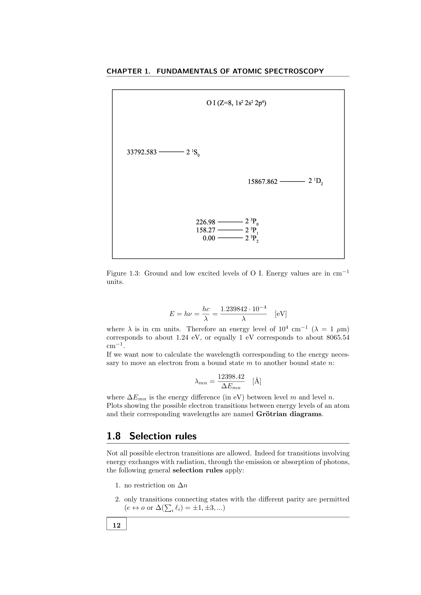
- [[Selection rules]] - $\Delta\ell = \pm 1$ for the jumping electron, $\Delta L = 0, \pm 1$ (not $0\to 0$), $\Delta J = 0, \pm 1$ (not $0 \to 0$), $\Delta S = 0$ (LS coupling), parity must change. electric dipole only.
- [[Forbidden vs permitted vs semiforbidden transitions]] - E1 (permitted), M1 + E2 (forbidden, $\sim 10^5$ to $10^8$ times weaker)
- Energy level diagrams Grötrian - plot of energy vs term, lines = allowed transitions
- [[Rydberg-Ritz formula]] - $\Delta E = R_H(1/n^2 - 1/m^2)$, $R_H = 13.6$ eV
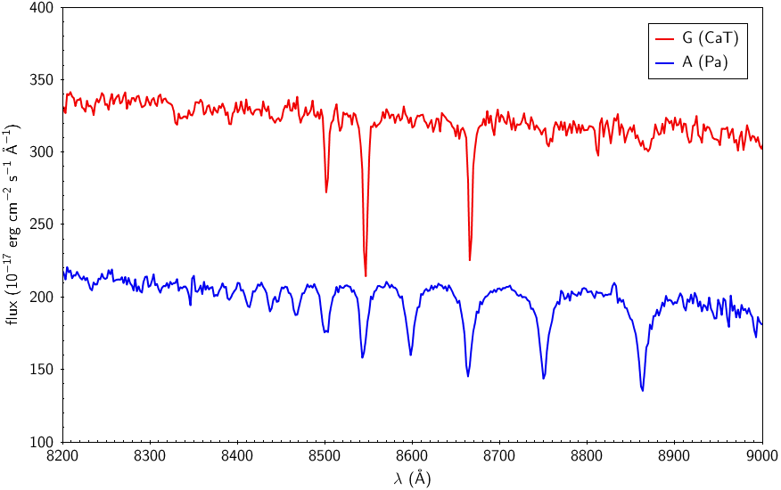
- [[Hydrogen spectral series]] - Lyman ($n = 1$, UV), Balmer ($n = 2$, optical), Paschen ($n = 3$, NIR), Brackett ($n = 4$, NIR)
- [[Helium energy levels]] - singlet ($S = 0$, parahelium) vs triplet ($S = 1$, orthohelium), $1s^1 2s^1$, $1s^1 2p^1$ etc.
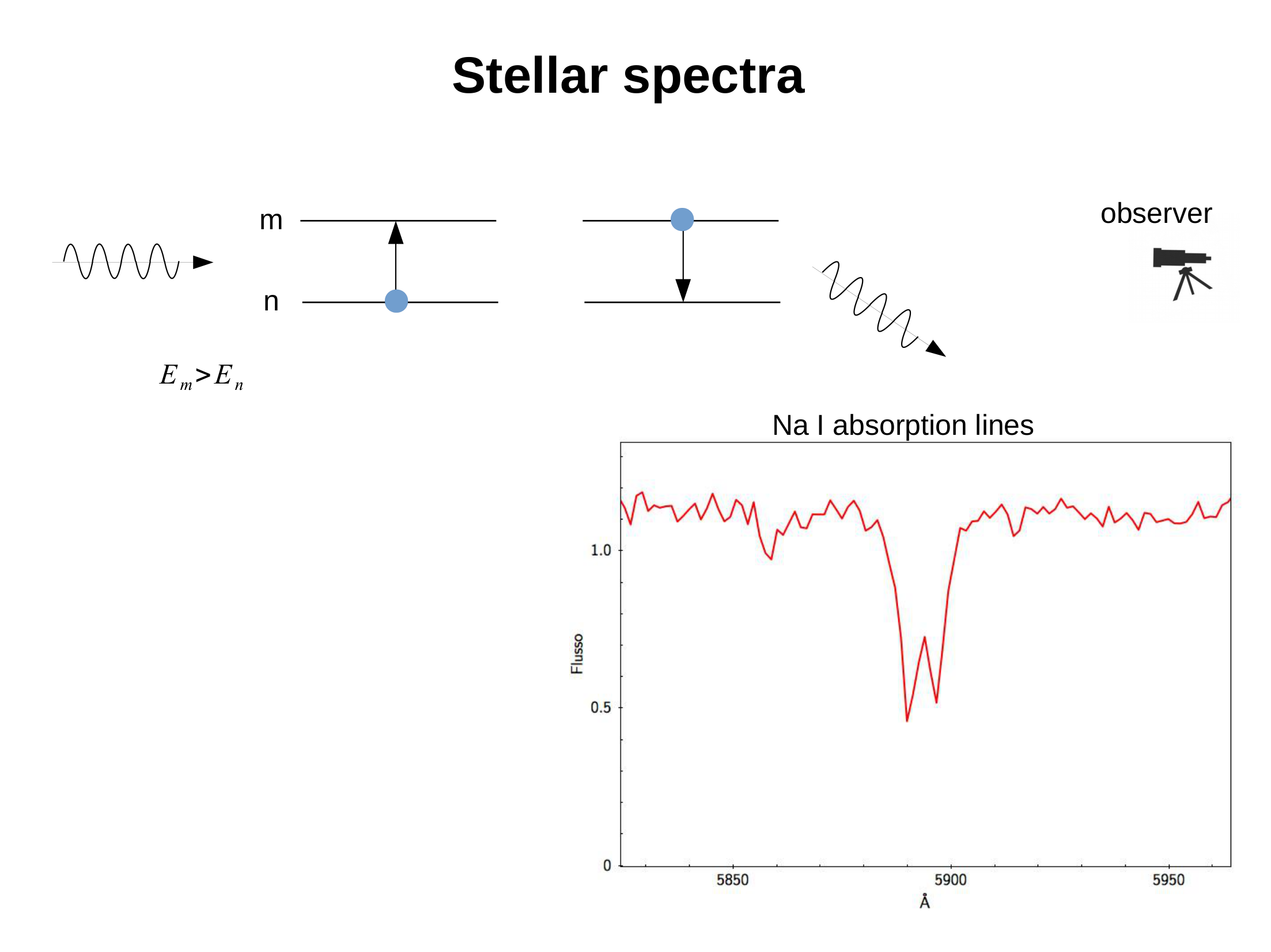
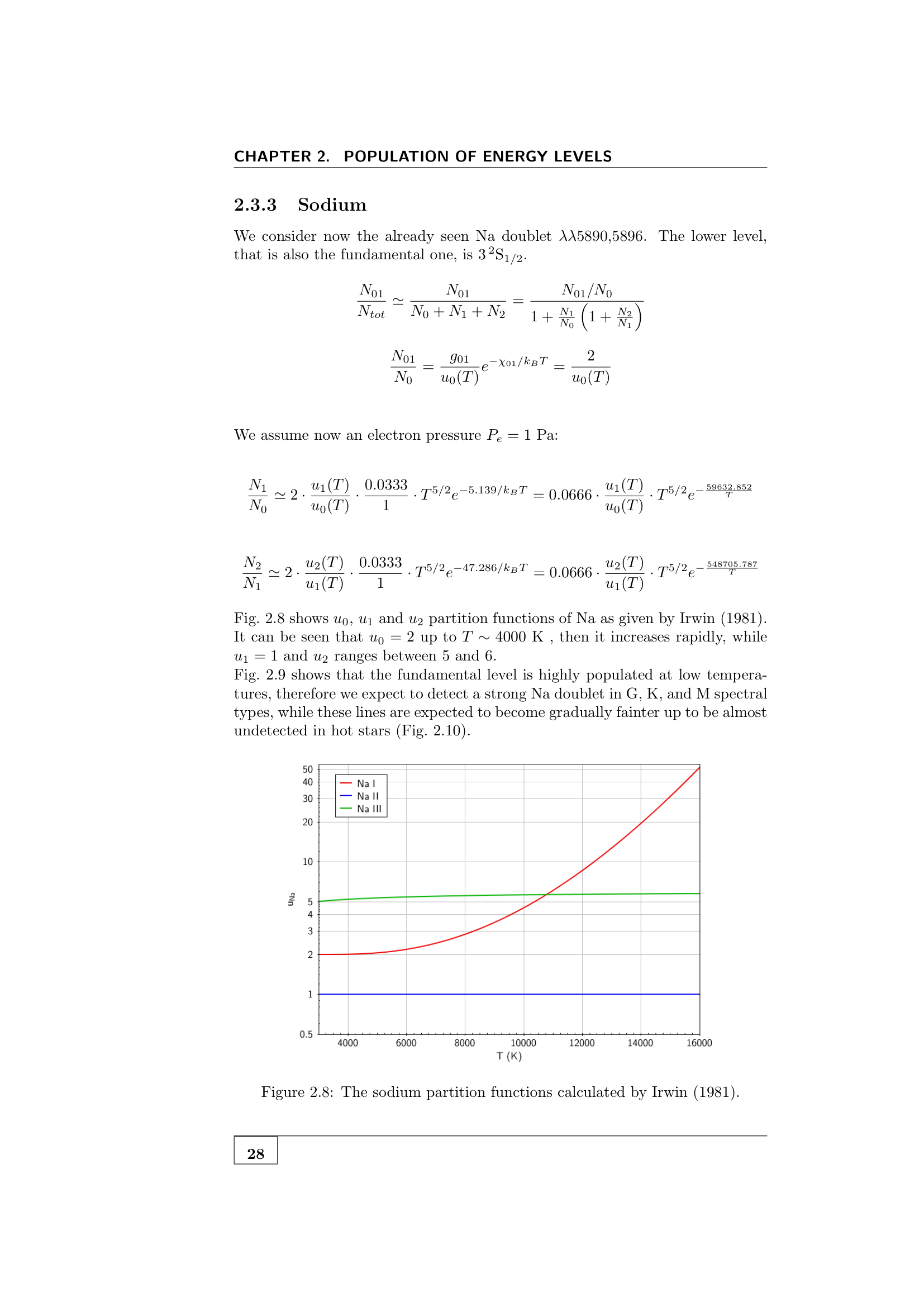
- [[Sodium and alkalis]] - $3s^1$ ground, D-doublet at $5890, 5896$ Å from $3p \to 3s$
- [[Magnesium and alkali earths]] - ground $1\,^1!S_0$, b-triplet near $5170$ Å from $3p\,^3P \to 3s\,^3S$
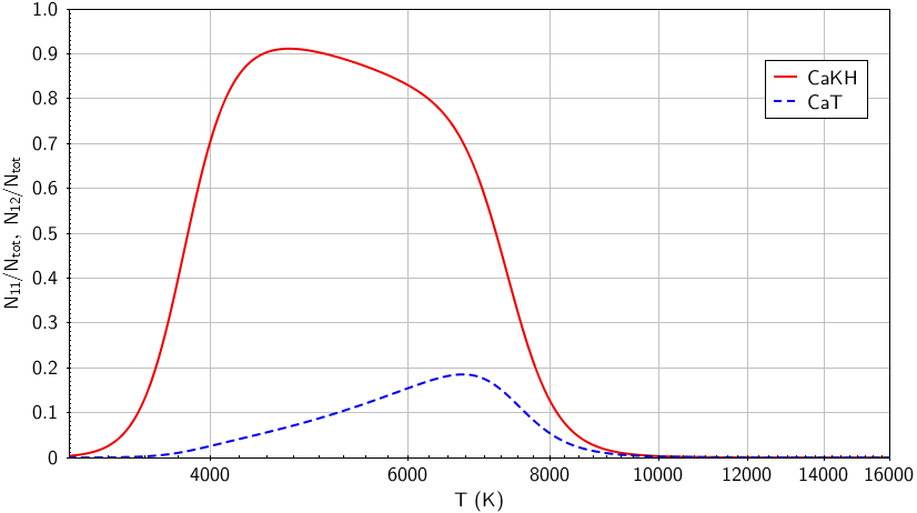
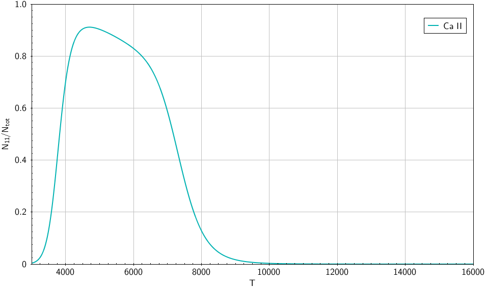
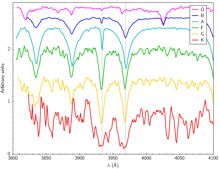
- [[Calcium and CaII H+K]] - single-electron ion, $4s^1 \to 3p^6 4s^1$ ground, K $3934$ Å, H $3968$ Å, very strong in cool stars
Block 3 - population of energy levels
a spectral line has strength $\propto$ number of atoms in the lower level. so to predict a spectrum I need to know how atoms distribute themselves across levels and ionisation stages. this block is the statistical-mechanics input.
- [[Boltzmann equation in spectroscopy]] - $n_i/n_j = (g_i/g_j) e^{-(E_i - E_j)/k_BT}$, populations within an ion at given $T$
- [[Saha ionisation equation]] - $n_{i+1} n_e/n_i = (g_{i+1}/g_i)\,(2\pi m_e k_B T/h^2)^{3/2}\, e^{-\chi/k_BT}$, ratio of two adjacent ionisation stages
- [[Partition function]] - $Z = \sum g_i e^{-E_i/k_BT}$, full statistical weight at temperature $T$
- [[Population of excited levels]] - Boltzmann + Saha together give $n_{ij} =$ (state $j$ of ion $i$). function of $T$, $n_e$
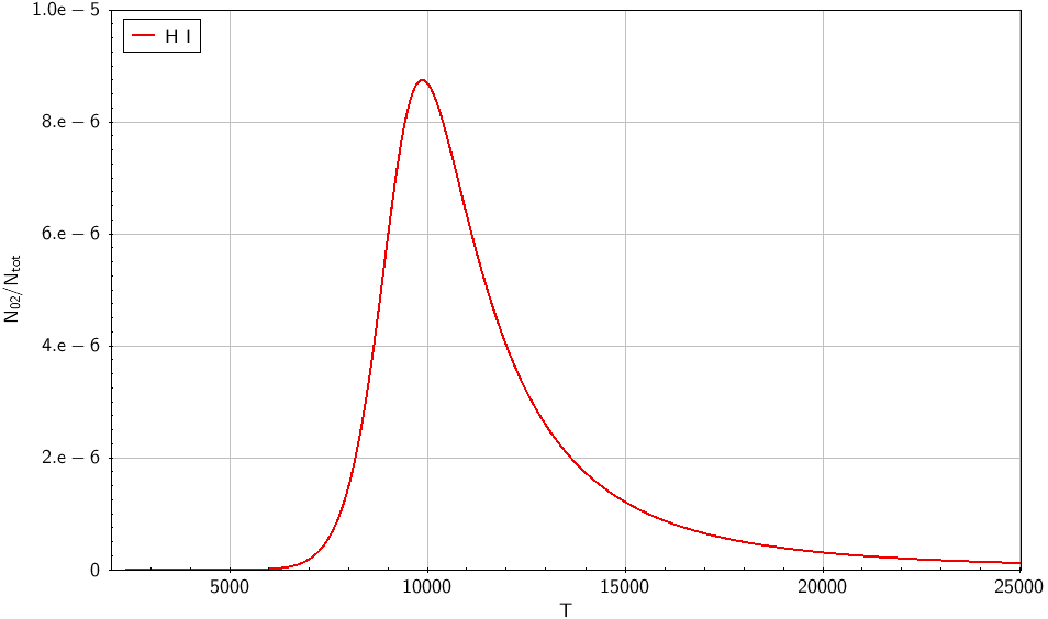
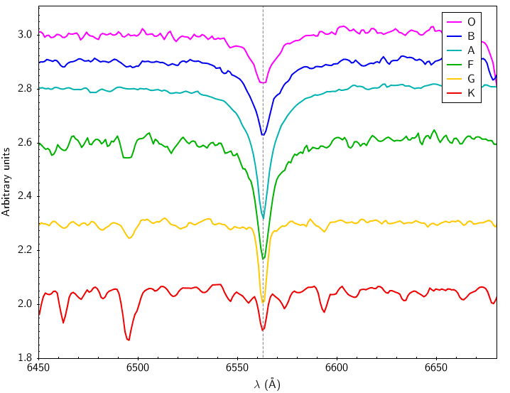
- [[Hydrogen population vs T]] - H I lines maximised at $T \sim 10\,000$ K (A0 stars), Saha competes with Boltzmann
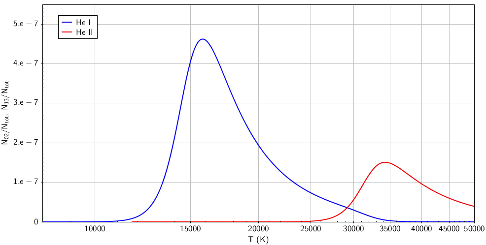
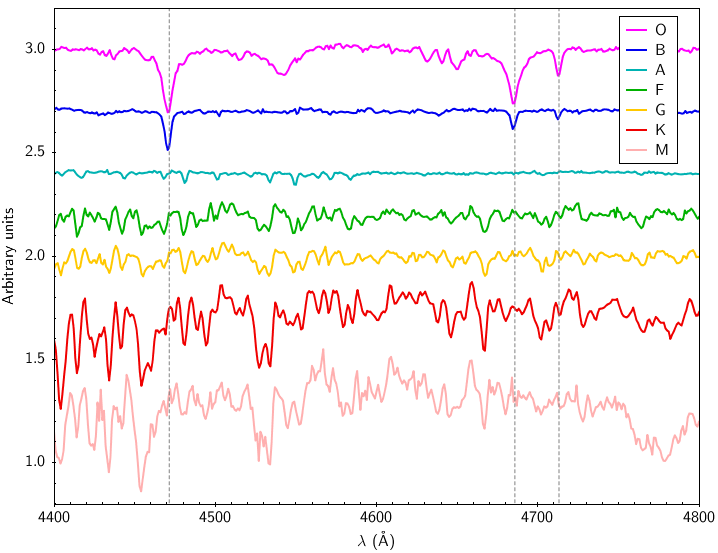
- [[Helium population vs T]] - He I and He II line strengths as $T$ thermometers in O and B stars
- [[Sodium population vs T]] - Na I D lines saturate at low $T$ (cool stars)
- [[Magnesium population vs T]] - Mg I b in cool stars, Mg II h+k in UV for hotter
- [[Calcium population vs T]] - Ca II K shows up at intermediate $T \sim 5000$ K
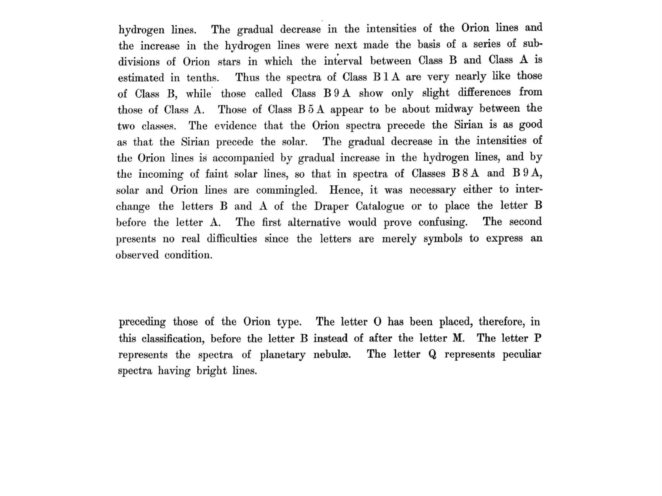
- [[Why the Sequence OBAFGKM]] - the line-strength patterns of these elements, plotted vs $T$, naturally generate the OBAFGKM ordering. this is the main result of Cecilia Payne’s 1925 thesis.
Block 4 - radiation transport
photons emitted somewhere in a hot gas are absorbed and re-emitted on their way out. the equation of radiative transfer describes this. this block sets up the formalism for stellar atmospheres specifically.
- [[Equation of radiative transfer]] - $dI_\nu/ds = -\kappa_\nu I_\nu + j_\nu$, absorption $\kappa$ and emission $j$
- [[Optical depth]] - $\tau_\nu = \int \kappa_\nu ds$, formal solution $I_\nu(\tau) = I_\nu(0) e^{-\tau} + \int_0^\tau S_\nu(\tau’) e^{-(\tau - \tau’)} d\tau’$
- [[Source function]] - $S_\nu \equiv j_\nu/\kappa_\nu$, in LTE $S_\nu = B_\nu(T)$
- [[Local thermodynamic equilibrium LTE]] - populations follow Boltzmann + Saha at the local $T$, valid where collisions dominate radiation
- [[Eddington-Barbier approximation]] - $I_\nu(0) \approx S_\nu(\tau = 1)$ for an emergent ray, the photon “sees” the layer at $\tau = 1$
- [[Limb darkening]] - at the limb of the Sun the line of sight crosses cooler outer layers, intensity drops
- [[Stellar atmosphere structure]] - photosphere, chromosphere, corona, $T(\tau)$ profile
- [[Continuum opacity sources]] - H$^-$ in cool stars, electron scattering in hot stars, bound-free absorption
Block 5 - absorption lines
how an absorption line forms, what shape it has, and what physical conditions broaden it. this block is the diagnostic-by-line-shape framework.
- [[Absorption coefficient and oscillator strength]] - $\kappa_\nu = (\pi e^2/m_e c)\, n_l\, f_{lu}\, \phi(\nu)$, $f$ = oscillator strength
- [[Line profile function phi nu]] - normalised $\int \phi(\nu)\,d\nu = 1$, sets the line shape
- [[Equivalent width]] - $W_\lambda = \int (1 - F_\lambda/F_c)\,d\lambda$, integrated absorption depth, dimensions of Å
- [[Curve of growth]] - $W$ vs column density $N$: linear regime $W \propto N$, logarithmic saturation, square-root damping wings
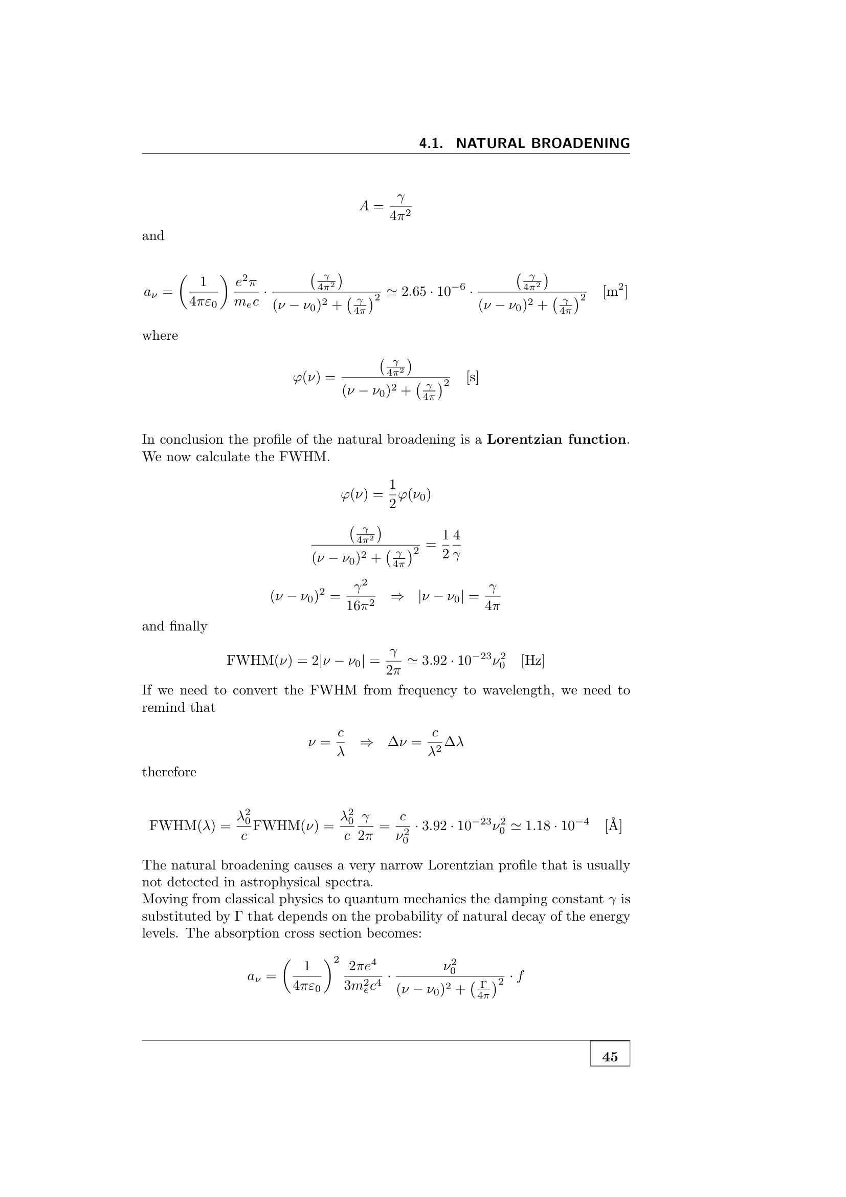
- [[Natural broadening Lorentzian]] - finite lifetime $\Delta E \cdot \Delta t \sim \hbar$, gives Lorentzian profile $\phi(\nu) \propto \gamma/[(\nu - \nu_0)^2 + (\gamma/2)^2]$
- [[Thermal Doppler broadening]] - Maxwell-Boltzmann velocity gives Gaussian profile, $\Delta\nu/\nu_0 = v_{\rm th}/c = \sqrt{2k_BT/m}/c$
- [[Microturbulence]] - extra Gaussian broadening above pure thermal, on scales smaller than the line-forming region
- [[Macroturbulence]] - large-scale velocity field, broadens but preserves equivalent width
- [[Collisional pressure broadening]] - perturbations from neighbouring particles, Lorentzian, $\propto P$ or $n_e$
- [[Stark broadening]] - special case of pressure broadening from electric microfields, dominant for H lines in hot stellar atmospheres
- [[Rotational broadening]] - stellar rotation $v\sin i$ broadens lines, characteristic shape with horns at $v\sin i$ from limbs
- [[Voigt profile]] - convolution of Lorentzian (natural + collisional) with Gaussian (thermal + turbulent), the standard line shape
- [[Damping wings]] - Lorentzian extension of Voigt at high column density, used to fit $\log gf$ from saturated lines
Block 6 - emission lines
in low-density photoionised gas, the line emission comes from collisional excitation, recombination cascades, and forbidden de-excitations. this block is the framework for HII regions, planetary nebulae, AGN narrow-line regions.
- [[Collisional excitation rate]] - $q_{lu} = \int v\,\sigma(v)\,f(v)\,dv$, function of electron $T_e$
- [[Statistical equilibrium equations]] - population balance: collisions up, collisions down, radiative decay
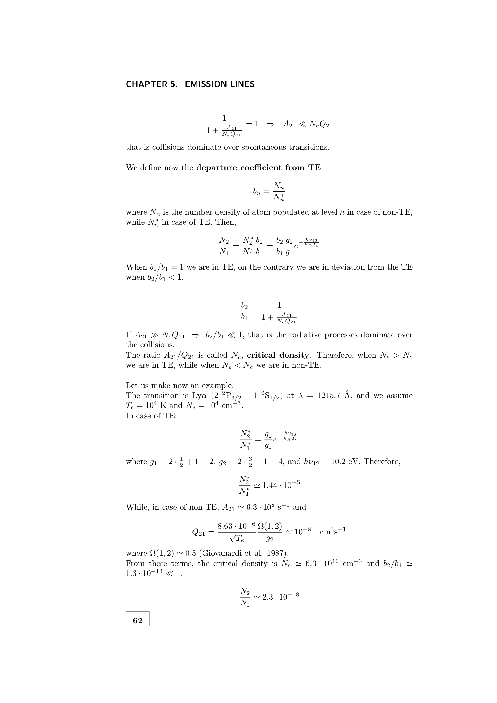
- [[Two-level atom]] - toy problem: collisional excitation balanced by radiative + collisional de-excitation, defines the critical density
- [[Critical density]] - $n_c = A_{ul}/q_{ul}$, transition from collision-limited to radiation-limited regime. forbidden lines have low $n_c$ (see below)
- [[Optically thin recombination lines]] - Case A vs Case B, $H\alpha/H\beta = 2.86$ in Case B at $T = 10^4$ K
- [[Case A vs Case B recombination]] - Case A: optically thin to Lyman lines (escape), Case B: optically thick to Lyman, $n \to 1$ transitions trapped, only Balmer and higher series escape
- [[Recombination line emissivity]] - $j_\nu \propto n_e n_p \alpha_{\rm eff}(T)$, weak $T$ dependence
- [[Forbidden lines]] - magnetic-dipole or electric-quadrupole transitions, very low $A_{ul}$, no spontaneous decay in laboratory
- [[OIII forbidden lines]] - $[OIII]\,\lambda 4959, 5007, 4363$ Å, the workhorse $T_e$ diagnostic via line ratio
- [[SII forbidden lines]] - $[SII]\,\lambda 6716, 6731$ Å doublet, the workhorse $n_e$ diagnostic
- [[Forbidden line diagnostics]] - $T_e$ from $\lambda 4363/(\lambda 4959+5007)$, $n_e$ from $\lambda 6716/\lambda 6731$, the two-tier nebular thermometer/densitometer
- [[Dust extinction in nebulae]] - Balmer decrement $H\alpha/H\beta$ vs $2.86$ measures $A_V$ along the line of sight
- [[Dilution factor]] - at distance $r$ from the central star, the radiation field is diluted by $W = (R_\star/r)^2/4$, used in low-density regions
Block 7 - continuum sources
emission and absorption of the continuum in stellar atmospheres and ionised gas. each mechanism has a distinct spectral signature.
- [[Recombination continuum]] - free electron + ion $\to$ atom + photon. emissivity $j_\nu \propto n_e n_i T_e^{-1/2}$ above the recombination edge $h\nu \ge \chi$
- [[Balmer continuum]] - recombination of H to $n = 2$, edge at $3646$ Å, dominant nebular UV continuum
- [[Free-free continuum]] - $\equiv$ thermal bremsstrahlung. $j_\nu \propto n_e n_i T_e^{-1/2}$ exponentially cut off at $h\nu \sim k_B T_e$. see [[Bremsstrahlung]]
- [[Synchrotron continuum]] - relativistic electrons in B-field, power-law spectrum $F_\nu \propto \nu^{-\alpha}$ with $\alpha \sim 0.5$ to $1$. see [[Synchroton]]
- [[Two-photon emission]] - H I 2$s$ $\to$ 1$s$ via $2\gamma$, gives a smooth UV continuum, important in nebular UV
- [[Thermal continuum from stellar photosphere]] - approximately Planck $B_\nu(T)$, modulated by H$^-$ opacity in cool stars
Block 8 - ionisation equilibrium
balance of photoionisations and recombinations in a photoionised cloud. determines the ionisation state of every species.
- [[Photoionization rate]] - $\Gamma = \int_{\nu_0}^\infty (4\pi J_\nu/h\nu)\,\sigma_\nu\,d\nu$ where $\sigma_\nu$ is the bound-free cross section
- [[Collisional ionisation rate]] - $C \propto n_e\,T^{1/2}\,e^{-\chi/k_BT}$, important in collisionally ionised plasmas (corona, SNR shocks)
- [[Recombination rate]] - $\alpha_A(T) = \int v\sigma_{\rm rec}(v) f(v)\,dv$, sums over all final levels (Case A) or excludes ground (Case B)
- [[Photoionisation balance]] - $n_X^{i+1} n_e \alpha = n_X^i \Gamma + n_X^i n_e C$, solve for ion fraction
- [[Ionisation parameter U]] - $U = Q_{H,\rm ion}/(4\pi r^2 n_H c)$, dimensionless ratio of photons to atoms
Block 9 - ionisation structure
once the ionisation balance per cell is known, the spatial structure of an ionised region follows. the canonical case is the Strömgren sphere.
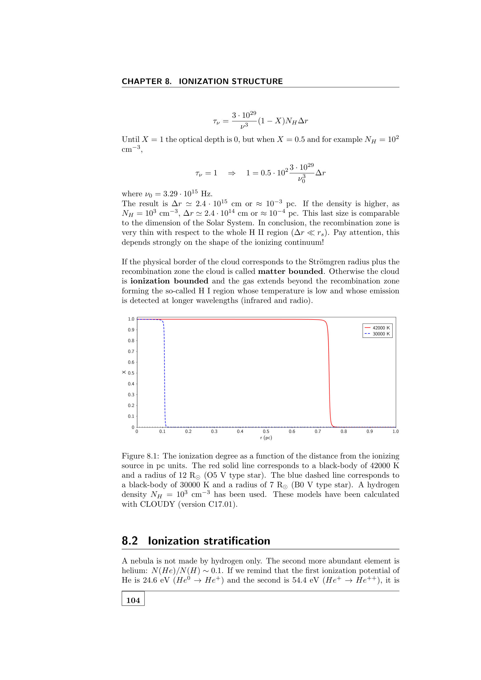
- Strömgren sphere - sphere of fully ionised H around an O star, radius $R_S = (3 Q_{H,\rm ion}/(4\pi n_H^2 \alpha_B))^{1/3}$, sharp boundary
- Strömgren sphere derivation - equate ionising photons emitted by the star to recombinations integrated over the sphere
- [[Ionisation stratification]] - at fixed $r$, different species are ionised to different stages (HII inside, OII just outside, OIII deeper, etc.)
- [[H I regions]] - neutral H surrounding the HII bubble, with He I, dust, and weak emission lines
- [[Photodissociation regions PDRs]] - neutral but warm boundary layers, FUV-dominated, [CII] + CO emission
- [[Ionisation parameter and ionisation state]] - $U$ controls which ions dominate, high $U$ gives high ionisation (O III, Ne III), low $U$ gives O II, S II
Block 10 - thermal equilibrium
what sets the temperature of an ionised gas? balance of heating (mainly photoelectric heating) and cooling (mainly forbidden-line emission).
- [[Heating rate in HII regions]] - $G \propto n_H \int \sigma_\nu (h\nu - \chi) (4\pi J_\nu / h\nu) d\nu$, from photoelectrons leaving energy in the gas
- [[Cooling rate in HII regions]] - $L \propto n_e n_X q_{lu}\,h\nu$, mainly from collisionally excited forbidden lines
- [[Equilibrium temperature]] - $G = L$ gives $T_e \sim 10^4$ K for typical HII regions, weakly dependent on density
- [[Cooling curve]] - $\Lambda(T) = L/n_e n_H$, has features at $\sim 10^4$ K (Ly$\alpha$), $\sim 10^5$ K (CIV, OVI), $\sim 10^7$ K (free-free)
Block 11 - applications, real-world spectra
object-by-object catalogue of what their spectra look like and what each line tells you. this is the part of the course that turns a lecture into a working diagnostic toolkit.
- [[Stellar spectra and spectral classification]] - OBAFGKM (existing note), the line strengths from Block 3 produce this sequence
- [[History of stellar classification]] - Secchi 1860s, Draper 1890, Pickering, Cannon, Payne 1925 (the temperature interpretation), MKK 1943, MK 1953
- [[MK luminosity classes]] - I (supergiants) to V (dwarfs), based on line widths reflecting surface gravity (pressure broadening)
- [[Emission line stars]] - Be stars (rotationally broadened H emission), WR stars (broad He II + N or C emission), T Tauri (accretion + emission)
- [[Galactic novae spectroscopy]] - V2491 Cyg as example, broad blueshifted absorption + emission, evolution over months
- [[Symbiotic star spectroscopy]] - cool giant + hot accreting WD, both signatures simultaneously, e.g. CI Cyg
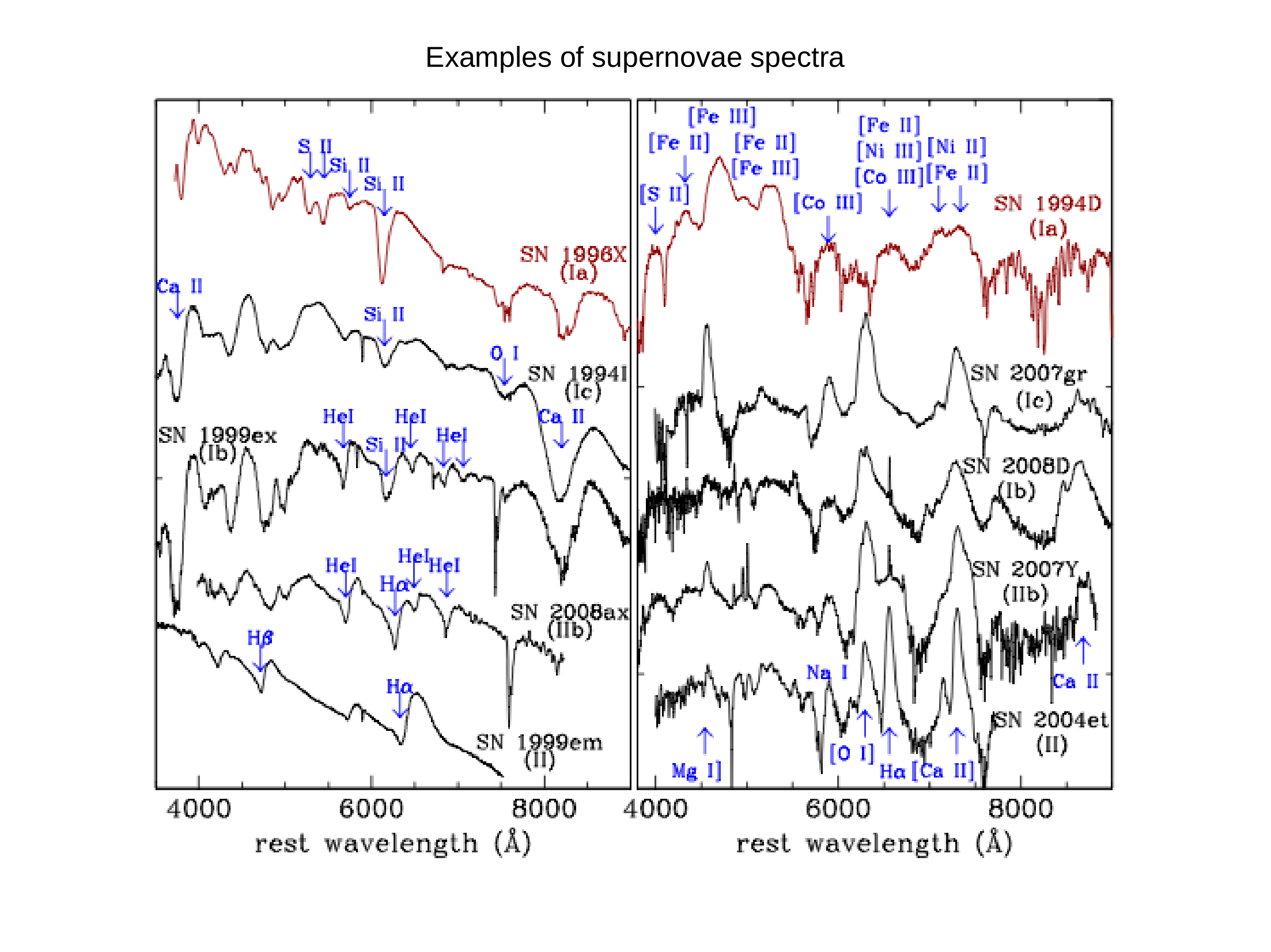
- [[Supernova spectroscopy]] - Type Ia (Si II $6355$ Å, no H), Ib (no H, He I), Ic (no H, no He), II (broad Balmer P-Cygni)
- [[H II region spectroscopy]] - strong Balmer + forbidden lines, faint continuum, weak metal absorption
- [[Planetary nebula spectroscopy]] - emission-line dominated, $[OIII]\,\lambda 5007$ very strong, central star may show Balmer absorption
- [[Supernova remnant spectroscopy]] - older SNR like Crab, M1: emission lines on faint continuum, [SII]/H$\alpha$ ratio diagnoses shock vs photoionisation
- [[Galaxy spectroscopy by type]] - elliptical (absorption-dominated, $4000$ Å break, Mg b, Na D, no emission), Sa (mixed), starburst (strong emission lines on blue continuum)
- [[AGN spectroscopy]] - Seyfert 1 (broad + narrow), Seyfert 2 (narrow only), LINER, BL Lac (featureless continuum), quasars (broad lines + featureless UV)
- [[BPT diagram]] - $[NII]/H\alpha$ vs $[OIII]/H\beta$ diagnostic separates star-forming galaxies from AGN
Block 12 - diagnostic toolkit
quick-reference summary of what each line ratio tells you. this is the “exam answer” version of the course.
- [[Spectroscopic Te diagnostics]] - $[OIII]\,\lambda 4363/(\lambda 4959+5007)$, $[NII]\,\lambda 5755/(\lambda 6548+6584)$
- [[Spectroscopic ne diagnostics]] - $[SII]\,\lambda 6716/\lambda 6731$, $[OII]\,\lambda 3729/3726$
- [[BPT diagram]] - galaxy classification (above)
- [[Balmer decrement]] - dust extinction (existing note)
- [[Spectroscopic redshift from line shifts]] - $z = (\lambda_{\rm obs} - \lambda_0)/\lambda_0$, several emission lines for cross-check
- [[Stellar velocity from Doppler shift]] - $v_r = c(\lambda_{\rm obs} - \lambda_0)/\lambda_0$, radial velocity surveys, exoplanets via $v \sin i$
- [[Velocity dispersion from line width]] - $\sigma_v$ in elliptical galaxies and clusters via line broadening
- [[Stellar v sin i from line shape]] - rotational broadening profile, $v\sin i$ from line-fit codes (rotbroad, ULySS)
- [[Curve of growth abundance analysis]] - log $gf$ + EW + atmospheric model $\to$ chemical abundances
Literature & Primary Sources
Canonical and modern arXiv astro-ph.SR/GA benchmark papers underlying the abundance-analysis and spectral-diagnostic techniques above.
- [[Asplund_2009_Chemical_Composition_of_the_Sun|Asplund et al. (2009) - The Chemical Composition of the Sun]] - 3D RHD solar abundance redetermination, solar modeling problem
- [[Nissen_Gustafsson_2018_High_Precision_Stellar_Abundances|Nissen & Gustafsson (2018) - High-Precision Stellar Abundances]] - differential line-by-line abundance methodology
- [[Maiolino_2024_JADES_Broad_Line_AGN_High_Redshift|Maiolino et al. (2024) - JADES Infant Black Holes at 4 < z < 11]] - JWST/NIRSpec broad-H$\alpha$ virial black-hole masses at high redshift
connections to other MOCs
- [[Observational_Astrophysics_MOC]] - the broadband / photometric counterpart. magnitudes count photons, spectroscopy resolves them.
- [[Fundamentals_Astrophysics_Cosmology_MOC]] - Block 2 (radiative mechanisms) and Block 5 (Saha + recombination) overlap with this course’s atomic-physics blocks.
- [[Observational_Cosmology_MOC]] - Block 9 (galaxy classification, AGN, line surveys) overlaps with this course’s Block 11.
- [[Lab_High-Energy_MOC]] - X-ray spectroscopy (CCD energy resolution, XRS, microcalorimeters) is a different waveband but the same concept.
- [[General_Relativity_MOC]] - only intersects via gravitational redshift (a small but real spectroscopic effect in white dwarfs and near black holes).
the exam-answer drafts I have
(none yet for this course, see Exams summer 2026 master plan phase 5 for when to build them.)
see also
- Moc - vault root MOC
- [[Spectroscopy_course_intro]]
- Exams summer 2026 master plan - Spectroscopy is exam #8, July 2026 (exact day TBC)
- [[Bremsstrahlung]]
- [[Synchroton]]
- [[Saha equation and recombination]] - the cosmological-recombination version
- [[Balmer decrement]]
- [[Stellar spectra and spectral classification]]
- [[Appendix D - Gratings and spectrographs]]
Master Figure Index (25 Total Images)
Every single spectral line population plot, observed stellar spectral comparison, spectrograph optical layout, and atomic transition diagram in 07_Images/Astronomical_Spectroscopy/ is cataloged below with direct links and pedagogical context:
| Image Asset | Diagnostic Category & Physics | Primary Zettel Note |
|---|---|---|
 |
Boltzmann-Saha ionization and excitation fractional population vs temperature curve | [[Stellar spectral types OBAFGKM]] |
 |
Boltzmann-Saha ionization and excitation fractional population vs temperature curve | [[Stellar spectral types OBAFGKM]] |
 |
Observed stellar spectral profiles across OBAFGKM sequence showing line strength variations | [[Stellar spectral types OBAFGKM]] |
 |
Observed stellar spectral profiles across OBAFGKM sequence showing line strength variations | [[Stellar spectral types OBAFGKM]] |
 |
Boltzmann-Saha ionization and excitation fractional population vs temperature curve | [[Stellar spectral types OBAFGKM]] |
 |
Observed stellar spectral profiles across OBAFGKM sequence showing line strength variations | [[Stellar spectral types OBAFGKM]] |
 |
Boltzmann-Saha ionization and excitation fractional population vs temperature curve | [[Stellar spectral types OBAFGKM]] |
 |
Observed stellar spectral profiles across OBAFGKM sequence showing line strength variations | [[Stellar spectral types OBAFGKM]] |
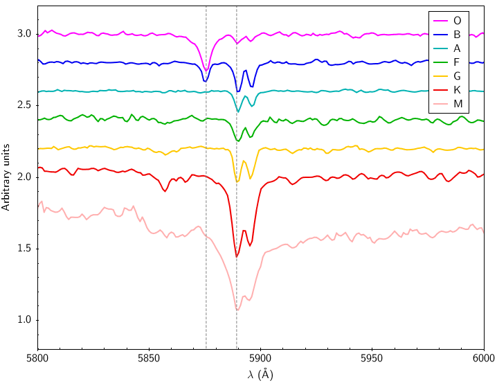 |
Observed stellar spectral profiles across OBAFGKM sequence showing line strength variations | [[Stellar spectral types OBAFGKM]] |
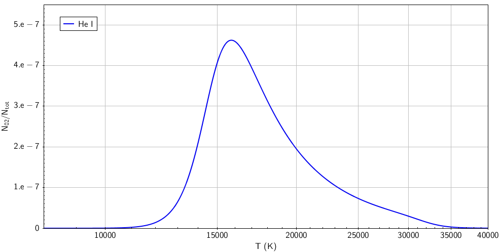 |
Boltzmann-Saha ionization and excitation fractional population vs temperature curve | [[Stellar spectral types OBAFGKM]] |
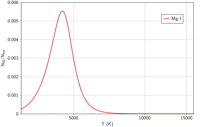 |
Boltzmann-Saha ionization and excitation fractional population vs temperature curve | [[Stellar spectral types OBAFGKM]] |
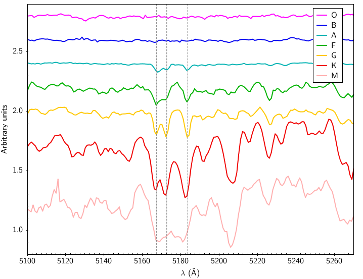 |
Observed stellar spectral profiles across OBAFGKM sequence showing line strength variations | [[Stellar spectral types OBAFGKM]] |
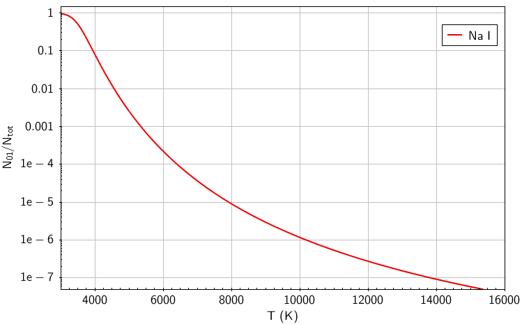 |
Boltzmann-Saha ionization and excitation fractional population vs temperature curve | [[Stellar spectral types OBAFGKM]] |
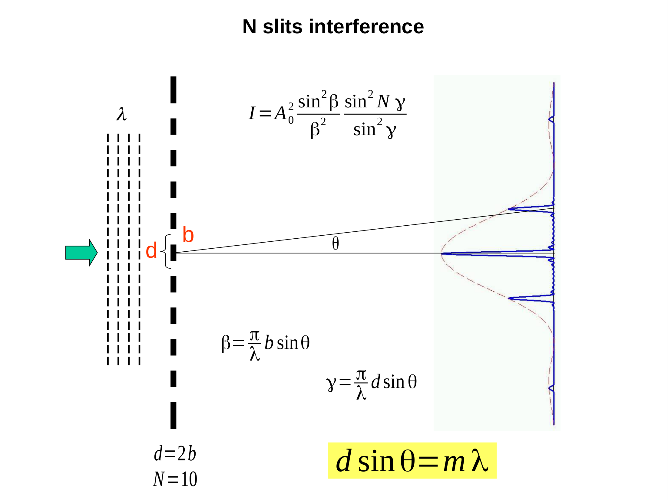 |
Spectrograph instrumentation: grating equation, blaze angle, dispersion, or echelle layout | [[Grating equation]] |
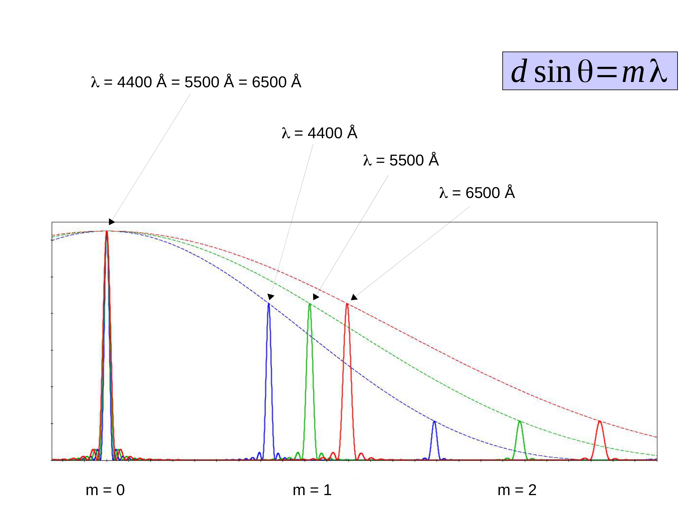 |
Spectrograph instrumentation: grating equation, blaze angle, dispersion, or echelle layout | [[Grating equation]] |
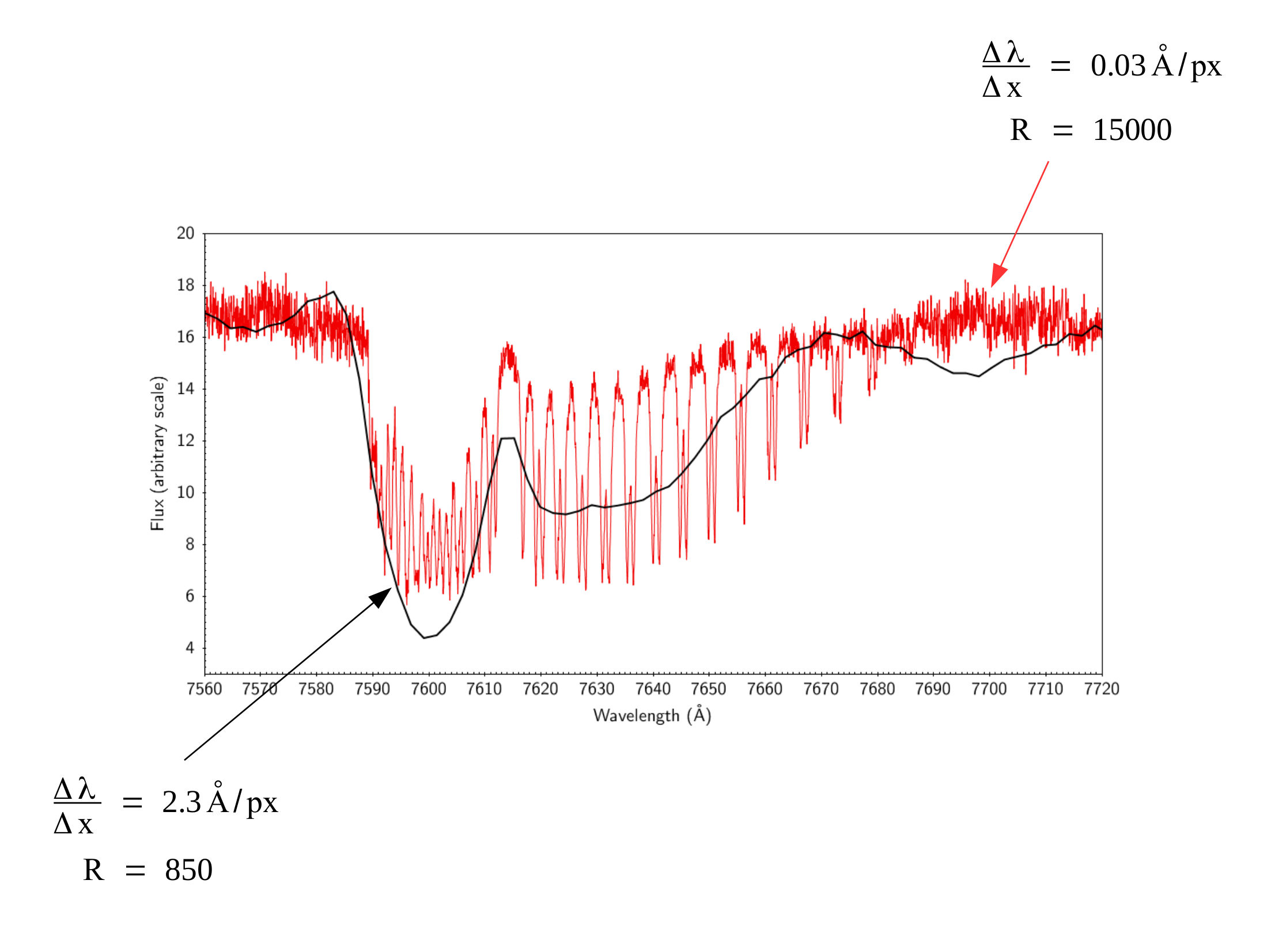 |
Spectrograph instrumentation: grating equation, blaze angle, dispersion, or echelle layout | [[Grating equation]] |
 |
Spectrograph instrumentation: grating equation, blaze angle, dispersion, or echelle layout | [[Grating equation]] |
 |
Spectrograph instrumentation: grating equation, blaze angle, dispersion, or echelle layout | [[Grating equation]] |
 |
Spectrograph instrumentation: grating equation, blaze angle, dispersion, or echelle layout | [[Grating equation]] |
 |
Atomic physics: LS coupling, selection rules, transition rates, curve of growth, or plasma diagnostics | [[Quantum numbers and atomic states]] |
 |
Atomic physics: LS coupling, selection rules, transition rates, curve of growth, or plasma diagnostics | [[Quantum numbers and atomic states]] |
 |
Atomic physics: LS coupling, selection rules, transition rates, curve of growth, or plasma diagnostics | [[Quantum numbers and atomic states]] |
 |
Atomic physics: LS coupling, selection rules, transition rates, curve of growth, or plasma diagnostics | [[Quantum numbers and atomic states]] |
 |
Atomic physics: LS coupling, selection rules, transition rates, curve of growth, or plasma diagnostics | [[Quantum numbers and atomic states]] |
 |
Atomic physics: LS coupling, selection rules, transition rates, curve of growth, or plasma diagnostics | [[Quantum numbers and atomic states]] |
Wikipedia and arXiv sources
Every zettel in this map ends with a short sourced section: a definition quoted from Wikipedia (118 zettels) or from the abstract of an arXiv review (6 zettels), and, where a free figure exists, the credited lead figure of the Wikipedia article (Wikimedia Commons) or a figure from an openly licensed arXiv paper. The lecture-slide figures above are unchanged.
| Zettel | Wikipedia | arXiv review | Figure |
|---|---|---|---|
| [[Absorption coefficient and oscillator strength]] | Oscillator strength | ||
| [[AGN spectroscopy]] | Active galactic nucleus | arXiv:1505.00811 | |
| [[Appendix D - Gratings and spectrographs]] | Diffraction grating | Commons | |
| [[Atomic term symbols]] | Term symbol | ||
| [[Balmer continuum]] | Balmer jump | Commons | |
| [[Balmer decrement]] | Balmer series | ||
| [[Blazed gratings]] | Blazed grating | ||
| [[Boltzmann equation in spectroscopy]] | Boltzmann distribution | Commons | |
| [[BPT diagram]] | Low-ionization nuclear emission-line region | arXiv:1910.09730 | Commons |
| [[Bremsstrahlung]] | Bremsstrahlung | Commons | |
| [[Calcium and CaII H+K]] | Fraunhofer lines | Commons | |
| [[Calcium population vs T]] | Saha ionization equation | ||
| [[Case A vs Case B recombination]] | Carrier generation and recombination | ||
| [[Collisional excitation rate]] | Collisional excitation | ||
| [[Collisional ionisation rate]] | Electron ionization | Commons | |
| [[Collisional pressure broadening]] | Spectral line | ||
| [[Continuum opacity sources]] | Opacity | Commons | |
| [[Cooling curve]] | Radiative cooling | ||
| [[Cooling rate in HII regions]] | H II region | arXiv:1910.09730 | Commons |
| [[Critical density]] | Forbidden mechanism | ||
| [[Curve of growth abundance analysis]] | Curve of growth | Commons | |
| [[Curve of growth]] | Curve of growth | Commons | |
| [[Damping wings]] | Spectral line shape | Commons | |
| [[Dilution factor]] | Inverse-square law | Commons | |
| [[Dispersion and spectral resolution]] | Spectral resolution | ||
| [[Dust extinction in nebulae]] | Extinction (astronomy) | Commons | |
| [[Echelle spectroscopy]] | Echelle grating | Commons | |
| [[Eddington-Barbier approximation]] | Limb darkening | Commons | |
| [[Emission line stars]] | Be star | Commons | |
| [[Equation of radiative transfer]] | Radiative transfer | ||
| [[Equilibrium temperature]] | Planetary equilibrium temperature | Commons | |
| [[Equivalent vs nonequivalent electrons]] | Electron configuration | Commons | |
| [[Equivalent width]] | Equivalent width | Commons | |
| [[Flux calibration]] | Spectrophotometry | Commons | |
| [[Forbidden line diagnostics]] | Forbidden mechanism | ||
| [[Forbidden lines]] | Forbidden mechanism | ||
| [[Forbidden vs permitted vs semiforbidden transitions]] | Selection rule | ||
| [[Free-free continuum]] | Bremsstrahlung | Commons | |
| [[Galactic novae spectroscopy]] | Nova | Commons | |
| [[Galaxy spectroscopy by type]] | Galaxy | Commons | |
| [[Grating equation]] | Diffraction grating | Commons | |
| [[H I regions]] | H I region | Commons | |
| [[H II region spectroscopy]] | H II region | arXiv:1910.09730 | Commons |
| [[Heating rate in HII regions]] | H II region | arXiv:1910.09730 | Commons |
| [[Helium energy levels]] | Helium atom | Commons | |
| [[Helium population vs T]] | Saha ionization equation | ||
| [[History of stellar classification]] | Stellar classification | Commons | |
| [[Hund’s rules]] | Hund’s rules | ||
| [[Hydrogen population vs T]] | Saha ionization equation | ||
| [[Hydrogen spectral series]] | Hydrogen spectral series | Commons | |
| [[Integral-field spectroscopy IFU]] | Integral field spectrograph | arXiv:1602.04267 | Commons |
| [[Ionisation parameter and ionisation state]] | Photoionization | Commons | |
| [[Ionisation parameter U]] | Photoionization | Commons | |
| [[Ionisation stratification]] | Strömgren sphere | Commons | |
| [[jj coupling]] | Angular momentum coupling | ||
| [[Limb darkening]] | Limb darkening | Commons | |
| [[Line profile function phi nu]] | Spectral line shape | Commons | |
| [[Local thermodynamic equilibrium LTE]] | Thermodynamic equilibrium | ||
| [[Macroturbulence]] | Spectral line shape | Commons | |
| [[Magnesium and alkali earths]] | Alkaline earth metal | ||
| [[Magnesium population vs T]] | Saha ionization equation | ||
| [[Microturbulence]] | Microturbulence | ||
| [[MK luminosity classes]] | Stellar classification | Commons | |
| [[Multi-object spectroscopy MOS]] | Optical spectrometer | Commons | |
| [[N-slit interference and gratings]] | Diffraction grating | Commons | |
| [[Natural broadening Lorentzian]] | Spectral line shape | Commons | |
| [[OIII forbidden lines]] | Forbidden mechanism | ||
| [[Optical depth]] | Optical depth | Commons | |
| [[Optically thin recombination lines]] | Emission spectrum | Commons | |
| [[Partition function]] | Partition function (statistical mechanics) | Commons | |
| [[Pauli principle and electron configurations]] | Pauli exclusion principle | ||
| [[Photodissociation regions PDRs]] | Photodissociation region | Commons | |
| [[Photoionisation balance]] | Photoionization | Commons | |
| [[Photoionization rate]] | Photoionization | Commons | |
| [[Planetary nebula spectroscopy]] | Planetary nebula | Commons | |
| [[Population of excited levels]] | Boltzmann distribution | Commons | |
| [[Quantum numbers and atomic states]] | Quantum number | Commons | |
| [[Recombination continuum]] | Carrier generation and recombination | ||
| [[Recombination line emissivity]] | Emission spectrum | Commons | |
| [[Recombination rate]] | Carrier generation and recombination | ||
| [[Rotational broadening]] | Stellar rotation | Commons | |
| [[Russell-Saunders LS coupling]] | Angular momentum coupling | ||
| [[Rydberg-Ritz formula]] | Rydberg–Ritz combination principle | ||
| [[Saha equation and recombination]] | Saha ionization equation | ||
| [[Saha ionisation equation]] | Saha ionization equation | ||
| [[Selection rules]] | Selection rule | ||
| [[SII forbidden lines]] | Forbidden mechanism | ||
| [[Single slit diffraction]] | Diffraction | Commons | |
| [[Sodium and alkalis]] | Alkali metal | ||
| [[Sodium population vs T]] | Saha ionization equation | ||
| [[Source function]] | Source function | ||
| [[Spectrograph design]] | Optical spectrometer | Commons | |
| [[Spectrograph types]] | Optical spectrometer | Commons | |
| [[Spectroscopic ne diagnostics]] | Plasma diagnostics | ||
| [[Spectroscopic redshift from line shifts]] | Redshift | Commons | |
| [[Spectroscopic Te diagnostics]] | Plasma diagnostics | ||
| [[Spectrum reduction pipeline]] | Astronomical spectroscopy | Commons | |
| [[Stark broadening]] | Stark effect | Commons | |
| [[Statistical equilibrium equations]] | Detailed balance | ||
| [[Statistical weight g]] | Degenerate energy levels | Commons | |
| [[Stellar atmosphere structure]] | Stellar atmosphere | Commons | |
| [[Stellar spectra and spectral classification]] | Stellar classification | Commons | |
| [[Stellar spectral types OBAFGKM]] | Stellar classification | Commons | |
| [[Stellar v sin i from line shape]] | Stellar rotation | Commons | |
| [[Stellar velocity from Doppler shift]] | Radial velocity | Commons | |
| [[Supernova remnant spectroscopy]] | Supernova remnant | Commons | |
| [[Supernova spectroscopy]] | Supernova | Commons | |
| [[Symbiotic star spectroscopy]] | Symbiotic binary | Commons | |
| [[Synchroton]] | Synchrotron radiation | ||
| [[Synchrotron continuum]] | Synchrotron radiation | ||
| [[Thermal continuum from stellar photosphere]] | Photosphere | Commons | |
| [[Thermal Doppler broadening]] | Doppler broadening | Commons | |
| [[Two-level atom]] | Two-state quantum system | Commons | |
| [[Two-photon emission]] | Two-photon absorption | Commons | |
| [[Velocity dispersion from line width]] | Velocity dispersion | ||
| [[Voigt profile]] | Voigt profile | Commons | |
| [[Wavelength calibration]] | Astronomical spectroscopy | Commons | |
| [[Why the Sequence OBAFGKM]] | Stellar classification | Commons |
Prof. Stefano Ciroi Oral Exam Defense Preparation Matrix
Question 1 - The Grating Equation, Angular Dispersion, and Resolving Power
- Blackboard Prompt: Derive the grating equation for a reflection grating. Derive the theoretical resolving power $R = \lambda/\Delta\lambda$ as a function of groove density $\rho$, order $m$, and illuminated width $W$. How does slit width limit actual resolution?
- Starting Equation: \(\sin\alpha + \sin\beta = \rho m \lambda = \frac{m\lambda}{d}\)
- Derivation & Blackboard Walkthrough:
- Consider parallel rays incident at angle $\alpha$ onto a grating with groove spacing $d = 1/\rho$. Diffracted rays leave at angle $\beta$.
- The optical path difference between rays diffracted from adjacent facets is: $\Delta = d\sin\alpha + d\sin\beta$. Constructive interference occurs when $\Delta = m\lambda$, yielding the grating equation.
- Differentiating with respect to $\lambda$ at fixed incidence $\alpha$ gives the angular dispersion: \(\cos\beta d\beta = \frac{m}{d} d\lambda \implies \frac{d\beta}{d\lambda} = \frac{m}{d\cos\beta} = \frac{\rho m}{\cos\beta}\)
- At the camera focal plane of focal length $f_{\rm cam}$, the linear dispersion is $\frac{dx}{d\lambda} = f_{\rm cam}\frac{d\beta}{d\lambda}$. The reciprocal linear dispersion is $P = \frac{d\lambda}{dx} = \frac{d\cos\beta}{m f_{\rm cam}}$.
- The diffraction limit of an aperture of width $W$ projected along the beam ($W\cos\beta$) sets the minimum angular separation (Rayleigh criterion): $\Delta\beta = \frac{\lambda}{W\cos\beta}$.
- Substituting into angular dispersion gives the theoretical resolving power: \(R_{\rm theo} = \frac{\lambda}{\Delta\lambda} = \lambda \frac{d\beta/d\lambda}{\Delta\beta} = \lambda \left(\frac{m}{d\cos\beta}\right) \left(\frac{W\cos\beta}{\lambda}\right) = m \frac{W}{d} = m N\) where $N = W/d$ is the total number of illuminated grooves.
- Slit-Limited Resolution: In practice, the entrance slit of physical width $s$ is projected onto the detector with magnification $M = f_{\rm cam}/f_{\rm coll}$. The projected slit width is $w_{\rm proj} = s \frac{f_{\rm cam}}{f_{\rm coll}} \frac{\cos\alpha}{\cos\beta}$. The actual resolving power is: \(R_{\rm slit} = \frac{\lambda}{\Delta\lambda_{\rm slit}} = \frac{\lambda}{w_{\rm proj} P} = \frac{\rho m W}{\alpha_{\rm slit} D_{\rm tel}}\) where $\alpha_{\rm slit} = s/f_{\rm tel}$ is the slit angular width on the sky.
Question 2 - The Boltzmann-Saha Balance and the Balmer Line Maximum in A-Stars
- Blackboard Prompt: Why are hydrogen Balmer absorption lines strongest in A0 stars ($T \approx 9,520$ K), and virtually vanish in both hot O-type stars ($T > 30,000$ K) and cool M-type stars ($T < 3,500$ K)? Derive the temperature of the maximum.
- Starting Equation: \(\frac{N_2}{N_{\rm total}} = \frac{N_2}{N_1}\frac{N_1}{N_0 + N_1 + N_2} \approx \frac{N_{1,2}}{N_1} \frac{N_1}{N_{\rm total}}\)
- Derivation & Blackboard Walkthrough:
- Balmer absorption lines (H$\alpha$, H$\beta$, etc.) originate exclusively from the $n=2$ excited level of neutral hydrogen H I.
- The fraction of neutral hydrogen atoms excited to $n=2$ is given by the Boltzmann equation: \(\frac{N_{1,2}}{N_{1,1}} = \frac{g_{1,2}}{g_{1,1}} e^{-\frac{E_2 - E_1}{k_B T}} = \frac{2(2)^2}{2(1)^2} e^{-\frac{10.2\,{\rm eV}}{k_B T}} = 4 e^{-\frac{1.184 \times 10^5}{T}}\) Because the excitation energy $\Delta E = 10.2$ eV is very high, at low temperatures ($T < 4,000$ K), virtually all atoms sit in the ground state $n=1$ ($N_{1,2}/N_1 \sim 10^{-13}$). Thus, cool stars have no Balmer lines.
- Conversely, the fraction of hydrogen that remains neutral is governed by the Saha ionization equation: \(\frac{N_{\rm II}}{N_{\rm I}} = \frac{2 k_B T}{P_e}\frac{u_{\rm II}}{u_{\rm I}}\left(\frac{2\pi m_e k_B T}{h^2}\right)^{3/2} e^{-\frac{\chi_{\rm ion}}{k_B T}}\) where $\chi_{\rm ion} = 13.6$ eV. At high temperatures ($T > 15,000$ K), hydrogen becomes almost completely ionized ($N_{\rm I}/N_{\rm total} \to 0$). Hot O and B stars have abundant free protons, but no neutral atoms to absorb Balmer photons!
- The population of the absorbing state is the product of Boltzmann excitation and Saha neutral fraction: $N_{1,2}(T) \propto e^{-10.2/kT} \left[1 + \frac{N_{\rm II}}{N_{\rm I}}\right]^{-1}$.
- Setting $\frac{d N_{1,2}}{dT} = 0$ for typical photospheric electron pressures $P_e \sim 20$ N/m$^2$ yields an exact peak at $T \approx 9,520$ K, corresponding precisely to spectral type A0V (Vega).
Question 3 - Plasma Diagnostics - Electron Temperature and Density from Emission Lines
- Blackboard Prompt: Explain how forbidden emission lines in photoionized gaseous nebulae (H II regions, planetary nebulae, AGN) determine electron temperature $T_e$ and electron density $n_e$. Derive the $[{\rm O\,III}]$ and $[{\rm S\,II}]$ line ratios.
- Derivation & Blackboard Walkthrough:
- In low-density nebular plasmas ($n_e \sim 10^2-10^4\,{\rm cm}^{-3}$), collisional excitation by thermal electrons is balanced by spontaneous radiative de-excitation and collisional de-excitation.
- Temperature Diagnostic ($[{\rm O\,III}]$):
- The $O^{2+}$ ion ($2p^2$ configuration) has a $^3P$ ground term, a $^1D_2$ metastable level at 2.51 eV, and a $^1S_0$ level at 5.35 eV.
- Transitions from $^1D_2 \to ^3P_{2,1}$ produce nebular green lines at $\lambda 5007$ and $\lambda 4959$ Å.
- Transition from $^1S_0 \to ^1D_2$ produces the auroral line at $\lambda 4363$ Å.
- The relative collisional excitation rate depends exponentially on the energy difference $\Delta E = E(^1S_0) - E(^1D_2) = 2.84$ eV: \(\frac{I(\lambda 4959 + \lambda 5007)}{I(\lambda 4363)} \approx \frac{7.9 \exp(3.29 \times 10^4 / T_e)}{1 + 4.5 \times 10^{-4}(n_e / \sqrt{T_e})}\)
- Because the exponential dependence on $T_e$ dominates, this ratio serves as an exquisite nebular thermometer ($T_e \sim 8,000 - 15,000$ K).
- Density Diagnostic ($[{\rm S\,II}]$):
- The $S^+$ ion ($3p^3$ configuration) has a $^4S_{3/2}$ ground state and two close excited levels: $^2D_{5/2}$ and $^2D_{3/2}$ at nearly identical excitation energies ($E \approx 1.84$ eV, $\Delta E \ll k_B T$).
- Spontaneous decay produces the doublet lines: $\lambda 6716$ Å ($^2D_{5/2} \to ^4S_{3/2}$, $A = 2.6 \times 10^{-4}\,{\rm s}^{-1}$) and $\lambda 6731$ Å ($^2D_{3/2} \to ^4S_{3/2}$, $A = 8.8 \times 10^{-4}\,{\rm s}^{-1}$).
- In the low-density limit ($n_e \ll n_{\rm crit} \sim 10^3\,{\rm cm}^{-3}$), every collisional excitation leads to a photon. The ratio reflects statistical weights: $\frac{I(6716)}{I(6731)} = \frac{g_1}{g_2} = \frac{6}{4} = 1.5$.
- In the high-density limit ($n_e \gg n_{\rm crit}$), collisional de-excitation thermalizes levels to Boltzmann distribution: $\frac{I(6716)}{I(6731)} = \frac{g_1 A_1}{g_2 A_2} = \frac{6(2.6)}{4(8.8)} \approx 0.44$.
- Between $n_e \sim 10^2$ and $10^4\,{\rm cm}^{-3}$, the ratio drops monotonically from 1.5 to 0.44, providing a clean nebular densitometer!
Essential Astronomical Spectroscopy Formulas Quick Sheet
| Law / Relation | Mathematical Formulation | Key Parameters & Diagnostics |
|---|---|---|
| Grating Equation | $m\lambda = d(\sin\alpha + \sin\beta)$ | $d = 1/\rho$ (groove spacing), $m$ (diffraction order) |
| Angular Dispersion | $\frac{d\beta}{d\lambda} = \frac{\rho m}{\cos\beta}$ | Rate of angular dispersion with wavelength |
| Reciprocal Linear Dispersion | $P = \frac{d\lambda}{dx} = \frac{d\cos\beta}{m f_{\rm cam}}$ | Å/mm or Å/pixel on CCD detector plane |
| Theoretical Resolving Power | $R_{\rm theo} = \frac{\lambda}{\Delta\lambda} = m N = \rho m W$ | Maximum diffraction-limited resolution of width $W$ |
| Slit-Limited Resolving Power | $R_{\rm slit} = \frac{\rho m W}{\alpha_{\rm slit} D_{\rm tel}}$ | Practical resolving power set by entrance slit angle $\alpha_{\rm slit}$ |
| Blaze Wavelength | $\lambda_B = \frac{2d}{m}\sin\theta_B \cos(\alpha - \theta_B)$ | Wavelength of maximum diffraction efficiency |
| Boltzmann Level Population | $\frac{N_b}{N_a} = \frac{g_b}{g_a} e^{-\frac{E_b - E_a}{k_B T}}$ | Thermal atomic level excitation ratio in LTE |
| Saha Ionization Equation | $\frac{N_{j+1}}{N_j} = \frac{2 k_B T}{P_e}\frac{u_{j+1}}{u_j}\left(\frac{2\pi m_e k_B T}{h^2}\right)^{3/2} e^{-\frac{\chi_j}{k_B T}}$ | Ionization stage population balance in photosphere |
| Equivalent Width Integral | $W_\lambda = \int \left(1 - \frac{F_\lambda}{F_{\rm cont}}\right) d\lambda$ | Integrated absorption line strength in Å |
| Curve of Growth (Linear) | $W_\lambda \propto N f \lambda^2$ | Optically thin regime ($\,\tau_0 \ll 1$) |
| Curve of Growth (Damping) | $W_\lambda \propto \sqrt{N f \gamma \lambda^4}$ | Strong pressure-broadened damping wings ($\,\tau_0 \gg 1$) |
| [O III] Temperature Ratio | $\frac{I(4959 + 5007)}{I(4363)} \approx 7.9 \exp(32900/T_e)$ | Electron temperature diagnostic in nebular plasmas |
| [S II] Density Ratio | $\frac{I(6716)}{I(6731)} \in [0.44, 1.50]$ | Electron density diagnostic between $10^2$ and $10^4\,{\rm cm}^{-3}$ |
Follow along on Instagram @your.astrophysicist · Report an issue